How to remove text in brackets along with brackets in Excel

Excel is beneficial when it comes to cleaning text data. Its powerful tools and functions enable users to clean, manipulate, and transform text-based information efficiently. With features like Find and Replace, Text-to-Columns, and a variety of text functions, Excel provides a versatile environment to remove unwanted characters, extract specific data, standardize formats, and perform various text-related operations.

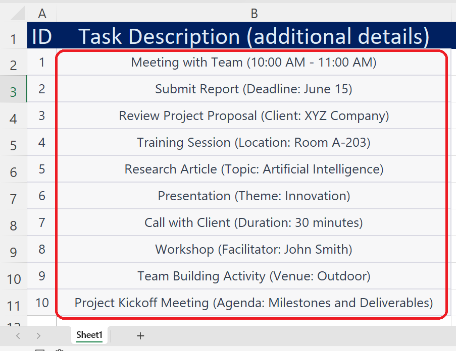
In today’s tutorial, we’ll learn how to remove unwanted or additional data which lies inside the brackets in Excel. Let’s examine our dataset which contains a list of task descriptions along with some additional information, which is useful only for you. Suppose you have to email this task list to someone else and you wish to remove all additional information from the list. The dataset is presented below;

Method 1: Use Flash Fill

Flash Fill is a powerful feature in Excel that helps automate data cleaning and transformation tasks. It uses intelligent pattern recognition to analyze the data and automatically fills in values based on the detected pattern. With Flash Fill, you can quickly extract, combine, or rearrange data without the need for complex formulas or manual data manipulation. However, Flash Fill works only when the data has no blanks and a clear pattern, otherwise, it will not work correctly. Furthermore, using the flash fill option, the original data will remain the same and the cleaned data will appear in a new column.

Step 1 – Create a sample data point for Flash Fill

• Change the header name of the column available just beside the dataset to “Task Descriptions”.
• In the first cell of the new column, write the data in the desired format i.e., after manually removing the unwanted or additional data as shown below.

Step 2 – Use the shortcut key to implement Flash Fill

• Now that the first data point is available, we can implement the Flash Fill method. To do this, use the shortcut key CTRL+E.
• This will detect the pattern in the data available in the left column, which is the original data column, and fill the whole column with the new pattern i.e., without the brackets as shown below.

Method 2: Use Find and Replace with the wildcard option

The Find and Replace tool in Excel is a powerful feature that becomes even more versatile when used with wildcards. Wildcards are special characters that represent patterns or unknown values in the search criteria, allowing for more flexible and advanced searches. We’ll use the asterisk * wildcard to detect the brackets and then delete them from all our data. Follow the steps mentioned below to learn how to do it using the Find and Replace tool. However, if we use this method this will change the original data and you don’t need to use any additional columns in this method. Therefore, if you want to delete the additional data permanently and retain only cleaned data, then you may use this method.

Step 1 – Open the Find and Replace dialog box

• Locate the Find and Select drop-down in the Editing group on the Home tab.
• Click on the drop-down menu and select Replace from the options. This will open the Find and Replace dialog box.
• Alternatively, you can use the shortcut key CTRL+H to open the same dialog box as shown below.

Step 2 – Write the search pattern with a wildcard

• Now type (*) in the Find what: field.
• Leave the Replace with: field blank as we wish to remove all the data inside the brackets along with the brackets.
• Press Replace All button to make changes in the data. You will see that the dataset will be cleaned as per our requirements as shown below.

Method 3: Use a combination of functions to remove data in brackets

We can also use a combination of three different functions to achieve the same goal. These functions are SUBSTITUTE, MID, and SEARCH. Together these functions will generate a customized formula that will remove the data inside the brackets along with the brackets. In this method, we’ll have to use another column again and the original data will remain as it is. Let’s follow the steps mentioned below to do it.

Step 1 – Select another column to get cleaned data

• Select another column right beside the dataset and change the name of the header to “Task Descriptions only” as shown below.

Step 2 – Write the combination of functions

• Write the following combination of functions in the very first cell after the header of the column, where we want to get cleaned data as shown below.

=SUBSTITUTE(B2,”(“&MID(B2,SEARCH(“(“,B2)+1,SEARCH(“)”,B2)-SEARCH(“(“, B2)-1) & “)”, “”).

The working of this formula will be explained at the end of the tutorial.

Step 3 – Implement the combination of functions to the whole data range

• Press the enter key to implement the formula in the first cell.
• After that, to implement the same formula to the whole dataset, use the fill handle. Either drag the fill handle down to the last data row or simply double-click the fill handle to copy the formula down the whole column as shown below.

Explanation of the combination of functions:

We have used the formula;

=SUBSTITUTE(B2,”(“&MID(B2,SEARCH(“(“,B2)+1,SEARCH(“)”,B2)-SEARCH(“(“, B2)-1) & “)”, “”).

This formula uses the SUBSTITUTE function along with the MID, SEARCH, and concatenation (&) functions to remove the data within brackets. Here’s how the formula works:

SEARCH(“(“, B2):

Finds the position of the opening parenthesis “(” within the text in cell B2.

SEARCH(“)”, B2):

Finds the position of the closing parenthesis “)” within the text in cell B2.

MID(B2, SEARCH(“(“, B2)+1, SEARCH(“)”, B2)-SEARCH(“(“, B2)-1):

Extracts the text between the opening and closing parentheses by using the MID function.

” (” & MID(B2, SEARCH(“(“, B2)+1, SEARCH(“)”, B2)-SEARCH(“(“, B2)-1) & “)”:

Creates a string that matches the exact text within the parentheses.

SUBSTITUTE(B2, ” (” & MID(B2, SEARCH(“(“, B2)+1, SEARCH(“)”, B2)-SEARCH(“(“, B2)-1) & “)”, “”):

Replaces the matched text (the data within parentheses) with an empty string, effectively removing it from the cell.