How to count a range of numbers in Excel
 By
SpreadCheaters
By
SpreadCheaters
Our dataset includes information about a grocery store’s bill, including the name and price of each product. We would like to determine the number of products within a certain price range. To accomplish this task, we will utilize the COUNTIFS function.
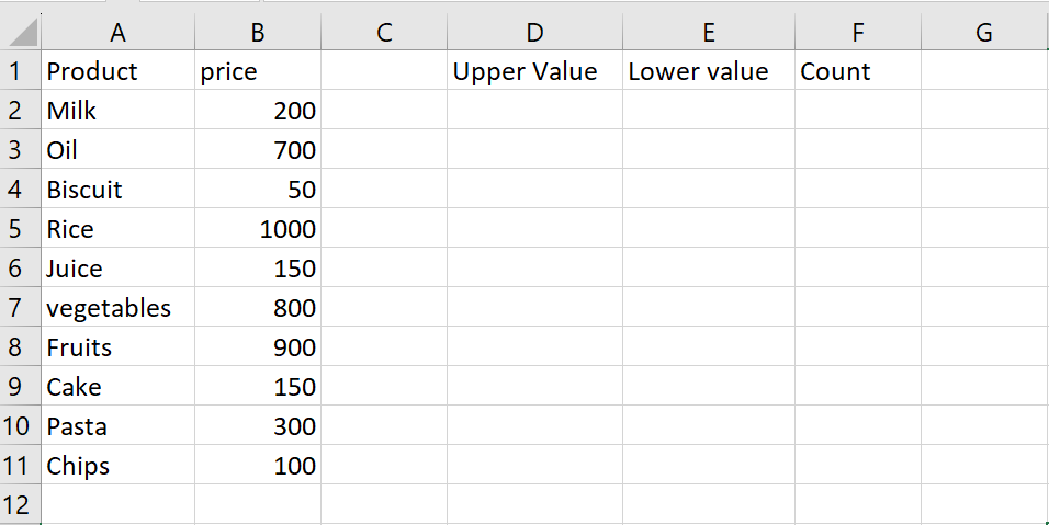

In Excel, counting a range of numbers means determining the total number of cells within a specific range that contains numerical values. Counting a range of numbers in Excel is a powerful tool that can help you make better use of your data and improve your overall results.
Step 1 – Select the Range
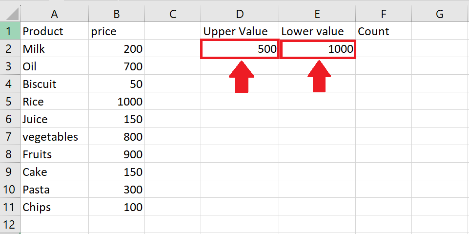
– Select the range of numbers between which you want to count
– To select the range type the lowest value and the highest values
– Here we have selected 500 as the lowest value and 1000 as the highest value
– You may select any other range
Step 2 – Select the Cell
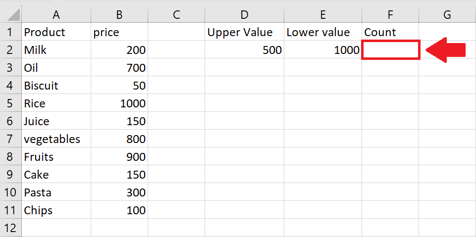
– After selecting the range, click on the cell where you want to show the count
Step 3 – Use the COUNTIF function
The COUNTIFS function in Excel is used to count the number of cells in a range that meet multiple criteria. It allows you to specify multiple criteria in different columns or the same column.
The syntax of the COUNTIFS function is:
– =COUNTIFS(criteria_range1, criteria1, [criteria_range2, criteria2], …)
criteria_range1: The range of cells that you want to apply the first criteria to.
criteria1: The first criteria that you want to apply to criteria_range1.
criteria_range2, criteria2: Additional ranges and criteria that you want to apply. You can specify up to 127 range/criteria pairs.
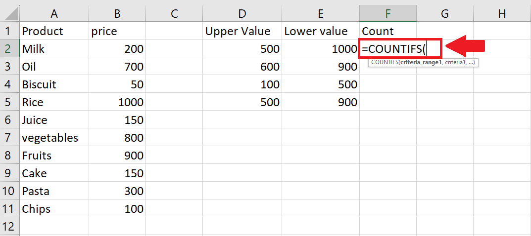
– After selecting the cell, use the COUNTIF function
– To use this function type “=COUNTIF(”
Step 4 – Type the Argument of the function
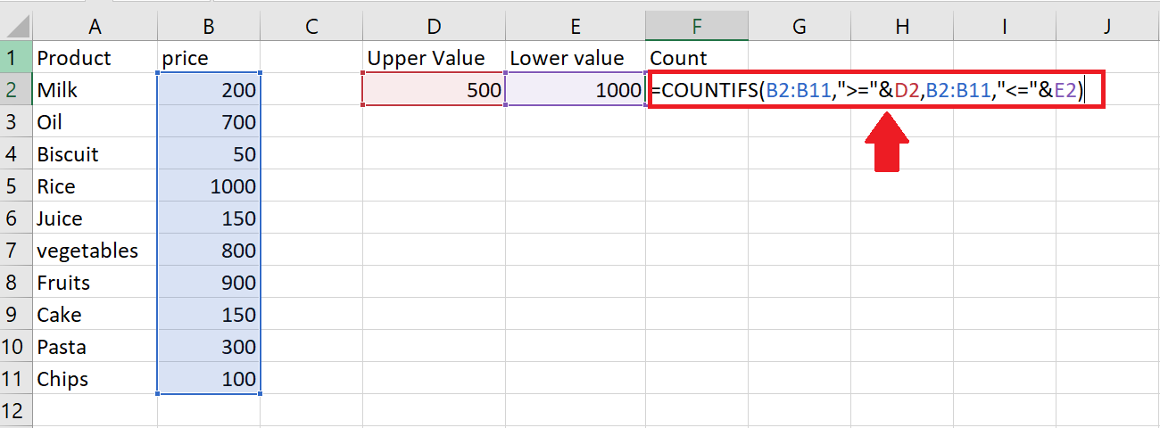
– After using the function, type the arguments as follows :
=COUNTIFS(B2:B11,”>=”&D2,B2:B11,”<=”&E2)
– The value in the cell is greater than or equal to the value in cell D2.
– The value in the cell is less than or equal to the value in cell E2.
– The “>=”&D2 and “<=”&E2 parts of the formula combine the comparison operators “>=” and “<=” with the cell references D2 and E2 using the ampersand (&) symbol. This creates text strings that the COUNTIFS function can use as criteria.
Step 5 – Press the Enter key
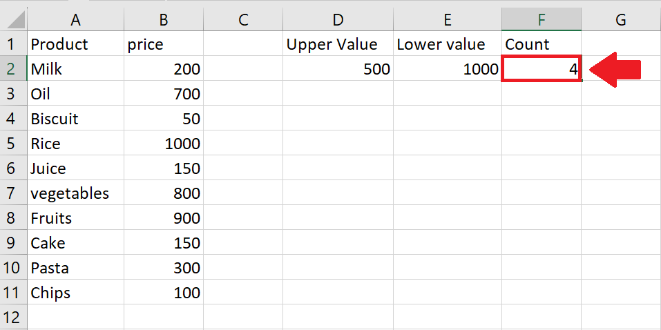
– After typing the formula, press the Enter key to get the required result
Step 6 – Apply on the Complete Column
– To apply on the complete column i.e count for different ranges, click on the cell where you have counted the range and a plus symbol will appear
– Click on this plus symbol and drag till the last cell you want