How to keep a running total in Google Sheets

In Google Sheets, maintaining a running total means consistently updating the sum or cumulative total of a sequence of numbers as new values are added or changed. This enables you to effortlessly monitor the current sum without the need to manually recalculate it every time a modification is made.

This tutorial will teach us how to keep a running total in Google Sheets. A running total in Google Sheets is used in various scenarios where you need to keep track of the cumulative sum of values over time. To save a running total we can use the method of anchoring cells or another method that includes utilizing the “Addition” operator.

Suppose we have a list of items that are being added to a grocery list. Our objective is to maintain a running total, which will provide us with the cumulative price that encompasses each product in the list.

Method 1: Keeping a Running Total by Anchoring Cells

An effective approach for maintaining a cumulative sum involves using the SUM function alongside a fixed reference to an initial cell. By anchoring the starting cell in the range, the ending cell adjusts accordingly, resulting in a running total.

Step 1 – Specify a Column for the Running Total

• Specify a separate column in which you want to keep the running total.

Step 2 – Utilize the SUM Function

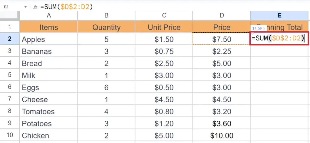
• Enter the SUM function.
• The structure will be as follows:

            SUM($A$2:A2)

• Here we have anchored the first reference i.e. $A$2 is a fixed cell reference.
• The reference A2 will update with the formula.
• Hit the Enter key.

Step 3 – Utilize Autofill to Apply the Function on the Column

• Utilize the Autofill feature to apply the function on the complete column.

Method 2: Utilizing the IF Function to Keep a Running Total

To maintain a continuous total, the IF function can be used as an Array formula, offering a highly efficient approach. By employing this method, the running total is automatically calculated and returned whenever a value is added. For this, we will use the following formula:

=IF(D2:D<>””,SUMIF(ROW(D2:D),”<=”&ROW(D2:D),D2:D),””)

Step 1 – Specify a Column for the Running Total

• Specify a separate column in which you want to keep the running total.

Step 2 – Utilize the Formula

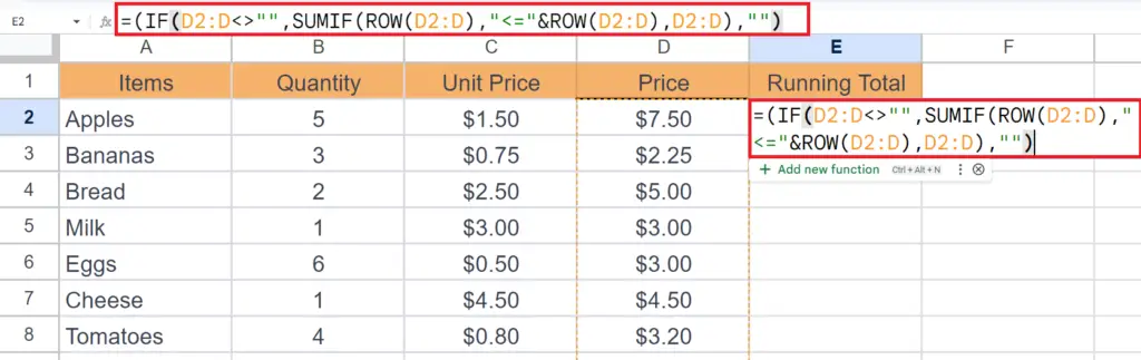
• Enter the Formula:

     =IF(D2:D<>””,SUMIF(ROW(D2:D),”<=”&ROW(D2:D),D2:D),””)

• The formula calculates a running total based on the values in column D.
• The First parameter of the IF function i.e. (D2:D<>””) checks if the cells in the range D2:D are not empty.
• It creates an array of row numbers corresponding to each cell in the range D2:D.
• The formula concatenates the “<=” operator with the row numbers to create an array of conditions.
• Using the SUMIF function, it sums the values in range D2:D based on the condition that the row number is less than or equal to the current row number.
• We have entered the complete range of the column i.e. D2:D, so that we can apply the function as an array formula.

Step 3 – Apply the Function as an Array Formula

• Apply the function as an array formula.
• For this, press the CTRL+SHIFT+ENTER keys.

Step 4 – Now Check the Running Total

• Now check the running total by adding more items to the list.
• The running total will automatically update.

Method 3: Keeping a Running Total Utilizing the Addition Operator

Another approach to keep a running total is by simply utilizing the addition operator. Below are the steps for this approach.

Step 1 – Specify a Column for the Running Total

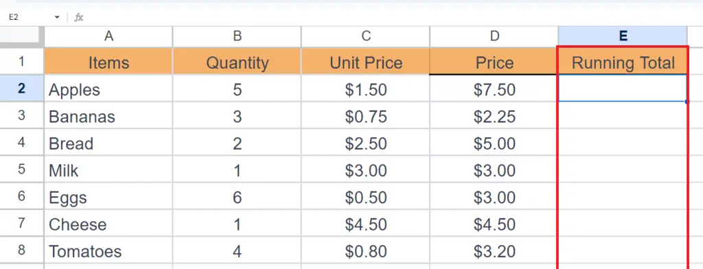
• Specify a separate column in which you want to keep the running total.

Step 2 – Copy and Paste the Price of the First Product

• Copy the price of the first product from the list utilizing the CTRL+C keys and paste it into the first cell of the targeted column by pressing CTRL+V.

Step 3 – Utilize the Addition Operator

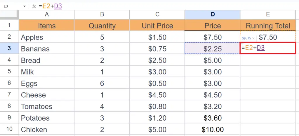
• Utilize the Addition operator in the next cell of the targeted column i.e. E2+D3.
• The cell E2 is the first cell of the targeted column i.e. in which we have placed the initial subtotal.
• Cell D3 is the cell containing the price of the second product.
• Hit the Enter key.

Step 4 – Apply the “Addition” operator Down the Column

• Apply the “Addition” operator down the column utilizing the Autofill feature.