How to change Google Sheets drop down list color
 By
SpreadCheaters
By
SpreadCheaters
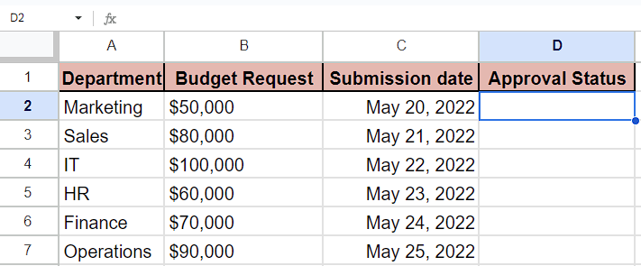
Let’s say that you are the financial manager of a company, and your responsibility is to review and approve or reject budgets submitted by various departments. You use Microsoft Excel to maintain a record of budget requests and track the approval or rejection status. Here is an example dataset illustrating this scenario:

A dropdown list in Google Sheets, also known as a data validation dropdown, is a feature that allows you to create a list of predefined options from which users can select a value. It provides a convenient and user-friendly way to ensure that data entered into a cell is limited to the options available in the dropdown list. You can change the color of the options in this data validation drop-down.
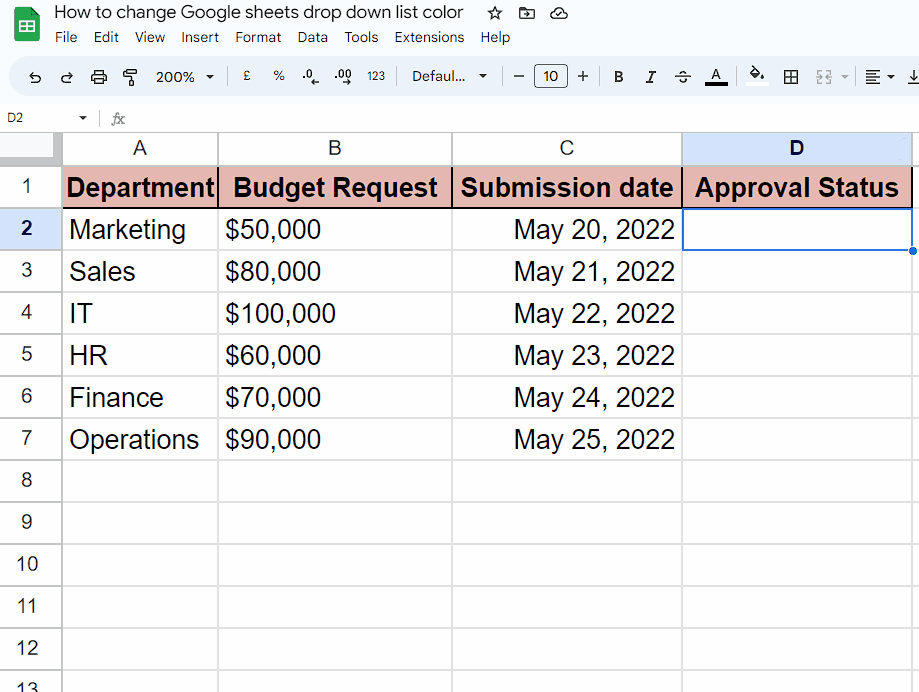
Step 1 – Selecting the cell
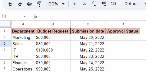
– Firstly, select an empty cell to which you want to add the drop-down list.
– We will teach you how to change the color of the drop-down list inserted in this cell later in this tutorial.
Step 2 – Inserting the drop-down list
– After selecting the cell, locate the Data tab and click on it and a list of options would appear on your screen.
– Then, click on the option named Data Validation.
– After clicking on the “Data Validation” option, a data validation rules box will open on the right side of your spreadsheet.
– You can also open this by Insert Tab or context menu.
Step 3 – Setting rules for the Drop-down list
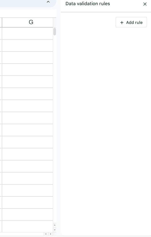
– In the data validation rules box, click on “Add a rule.”
– Then, write the range of cells in Apply to Range option. For example, it is D2:D7 in our case.
– Two boxes will appear under the criteria, labeled Option 1 and Option 2.
– You can rename these options according to your preference. For instance, we’re changing Option 1 to “Approved” and Option 2 to “Disapproved.”
– If you want to add more options, click on “Add another item” below the drop-down list options.
– In our example, we added another option and named it “Pending.
Step 4 – Changing the color of the Drop-down list
– Once you’ve set up rules for the drop-down list, locate the grey circle adjacent to the options which we have named.
– Click on this circle, and a box will appear with a variety of color options to choose from.
– Choose any color you like and this color would be assigned to the option that you’ve selected.
– Repeat the above step for changing the color of other options in the drop-down list.
– For instance, we’ve assigned green color to the option named “Approved”, red color to the option named Disapproved, and yellow color to the option named “Pending”.
– Then, click on any cell containing the drop-down list option, and click on it.
– Next, choose an option from the dropdown menu, and it would acquire the color corresponding to the selected option.