How to remove text between parentheses along with parentheses in Google Sheets

Google Sheets is a robust online spreadsheet tool that offers a wide range of functions and features to effectively manage and manipulate data. It proves particularly useful when dealing with data obtained from various sources, such as web pages, different office branches, or the output of data mining software. During such instances, it is common to encounter datasets containing extraneous information that needs to be eliminated through data cleansing.

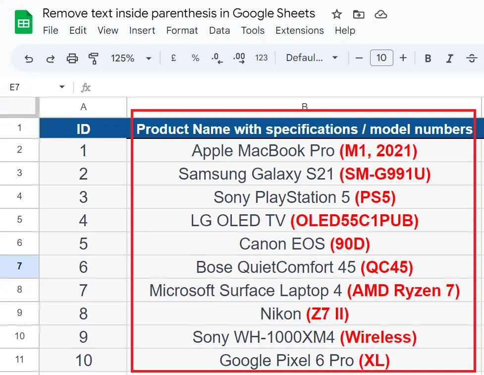
In today’s tutorial, we’ll learn a technique to remove unnecessary data inside the parenthesis. Our dataset contains the product names of different types of electronic devices and accessories. Each product name may have additional information enclosed in parentheses, such as specifications, color, or version details. This additional information has been marked in red color already, to show what needs to be removed. So, we’ll remove the details inside the parenthesis and keep the product names only. The dataset is presented below;

Let’s follow the methods and steps mentioned in these methods to learn how to extract the required data from this dataset.

Method 1: Use the Regular Expression function

Regular expressions (regex) are a powerful tool in Google Sheets for performing advanced data manipulation and pattern-matching operations. Using a specific regular expression, we can find any pattern inside the data. We can then use the match, replace or extract functions based on our requirements. However, you will need an extra column to use this function, and the original data will remain the same. Google Sheets provide the following three methods which can use regular expressions;

• REGEXMATCH(text, regular_expression)
• REGEXEXTRACT(text, regular_expression)
• REGEXREPLACE(text, regular_expression, replacement)

We will use the last one i.e. REGEXREPLACE(text, regular_expression, replacement) because we want to remove all the information inside the parenthesis. This function requires three arguments which are explained below;

text: This is the text data or any data upon which we wish to use the regular expression

regular_expression: This is the specific regular expression that will tell the function which data is to be replaced.

replacement: This is the text or any other data that will be used as a replacement for all data inside the parenthesis.

Step 1 – Select the cell and write the appropriate formula

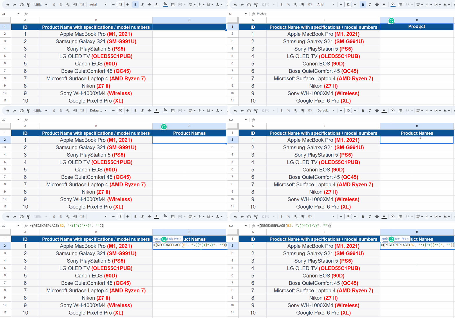
• Select an appropriate column outside the dataset and write “Product names” in the header of the column.
• In the next cell of the same column, write the following regular expression formula in that cell.

=(REGEXREPLACE(B2, “\([^()]*\)”, “”)

This is the formula that tells the Google Sheets function to find the data inside the parenthesis within cell B2 and replace it with a blank space.

Step 2 – Press Enter to implement the formula

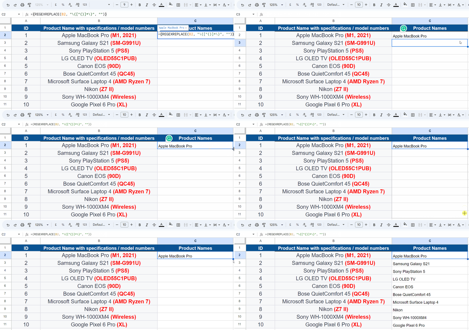
• After writing the formula, press the enter button from the keyboard to implement the formula. This will replace all the text inside the parenthesis and provide us with the desired results.
• To implement the formula to the whole range of data, you can drag it down the whole data range to implement the formula down the column or double-click the fill handle as shown below.

Method 2: Use Regular Expression with Find & Replace

We can use the same regular expression that we used in the last method along with Find & Replace tool to remove the data inside the parenthesis. This method will be useful if you don’t want to create an additional column and want to cleanse the original data only. Let’s follow the steps mentioned below to do it.

Step 1 – Open the find and replace tool

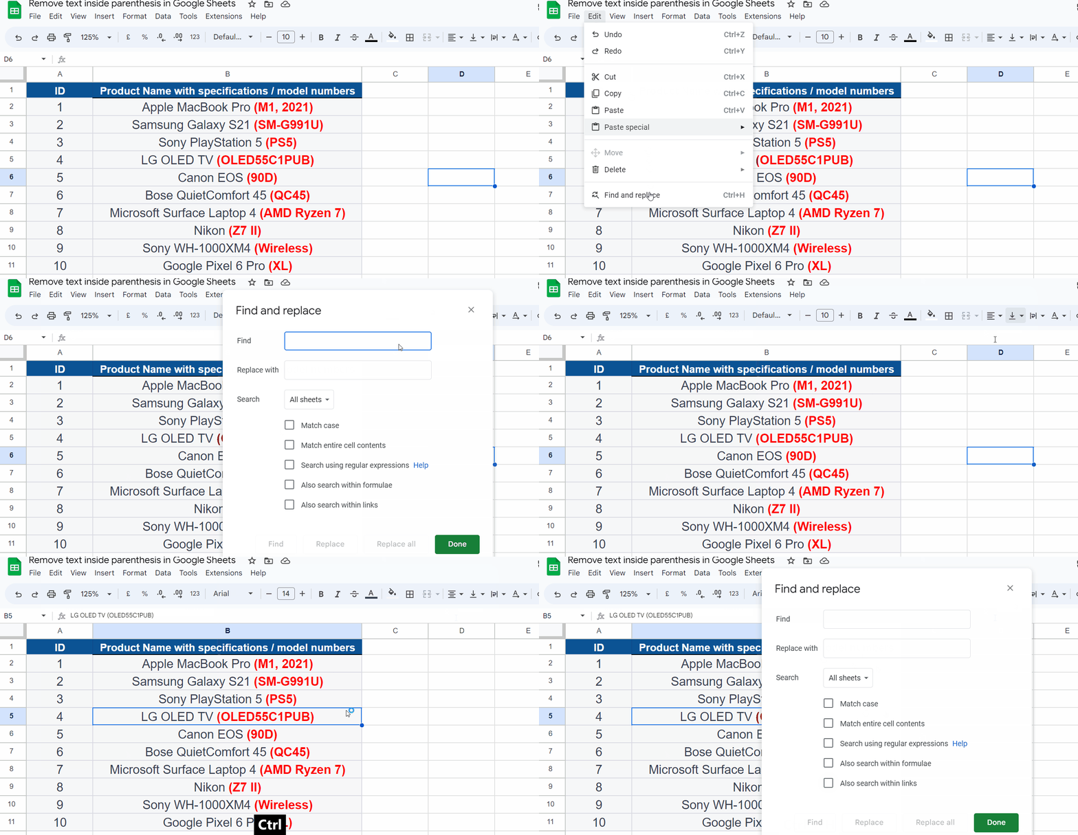
• Go to the Edit menu and click on it.
• A drop-down menu will appear. Locate the Find and Replace option and click on that to open the dialog box. 
• Alternatively, you can use the shortcut key CTRL+H to open the same dialog box.

Step 2 – Select the appropriate options to use Regular Expression

• In the Find and replace dialog box, check the tick box against “Search using regular expressions”. 
• This will automatically check the “Match case” option as well. We can uncheck this option if we don’t want to find only the exact matches but we’ll keep it checked as shown below.

Step 3 – Write the regular expression in the Find field

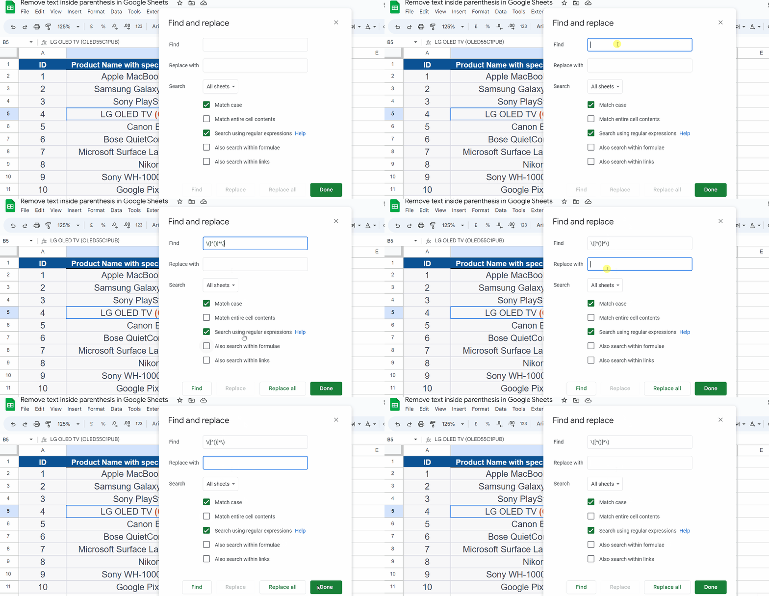
• Now write the following regular expression in the “Find” field;

\([^()]*\)

• Keep the “Replace with” empty as we wish to remove all the text inside the parenthesis.

Step 4 – Use Replace all option to remove the additional data

• If you have more than one sheet and you want to remove the data in the current sheet only then choose the “This Sheet” option from the “Search” drop-down field.
• Press the “Replace all” button to remove all the unnecessary data inside the parenthesis along with the parenthesis as well.

Explanation of the Regular Expression used:

The formula used, (REGEXREPLACE(B1, “\([^()]*\)”, “”), is a regular expression-based formula used in Google Sheets to remove text inside parentheses from a range of cells.

Let’s break down the formula:

B2: This refers to the cell you want to apply the formula to. It can be a single cell or a total column or a range of cells.

REGEXREPLACE: This is the function that performs the regex-based replacement in Google Sheets. It allows you to replace text that matches a specific regex pattern.

“\([^()]*\)”: This is the regular expression pattern used to match text inside parentheses. Let’s break it down further:

\(: Matches an opening parenthesis “(“.

[^()]*: This matches any characters that are not opening or closing parentheses. The [^()] is a negated character set, and * indicates zero or more occurrences of those characters.

\): Matches a closing parenthesis “)”.

Combining these parts together, the pattern “\([^()]*\)” matches any text enclosed in parentheses.

“”: This is the replacement text, an empty string (“”). In other words, it replaces the matched text (text inside parentheses) with nothing, effectively removing it from the cell.

By applying this formula to a range of cells in Google Sheets, you can remove the text inside parentheses from each corresponding cell in the range.