
How to do conditional formatting if another cell contains text in Google Sheets
 By
SpreadCheaters
By
SpreadCheaters
In our dataset, we have a list of students’ names along with their corresponding pass or fail status. Our goal is to apply conditional formatting to the names based on the status column. The following steps will guide you to perform this Conditional Formatting.
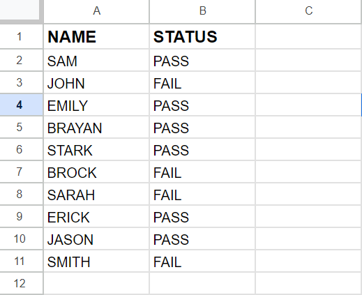
When using conditional formatting with the “Text contains” rule, you can specify a particular text string, and if that text is found within another cell, the formatting will be applied to the target cell. This feature helps you visually highlight or emphasize certain data based on the presence of specific text in another cell.
Step 1 – Select the Cell
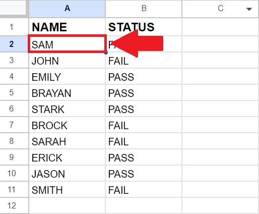
– Click on the cell that you want to format
Step 2 – Click on the Format tab
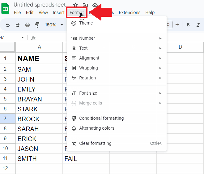
– After selecting the cell, click on the Format tab and a dropdown menu will appear
Step 3 – Click on the Conditional Formatting option
– Afterward, click on the Conditional formatting from the drop-down menu and a dialog box will appear
Step 4 – Click on the Custom Formula Is option
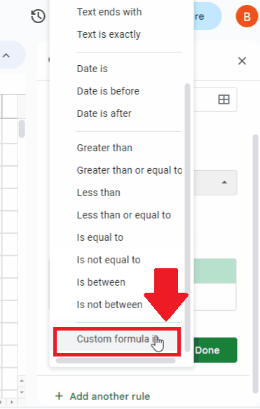
– Click on the “Custom formula is” option from the box below the Format Cells If the option.
Step 5 – Type the Formula
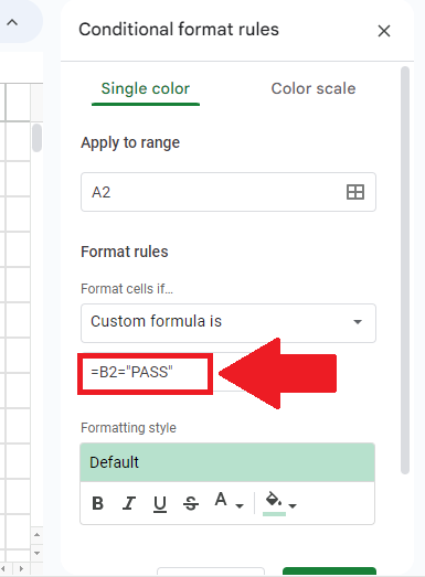
– Type the following Formula in the Value or Formula option box:
=B2=“PASS”
– You may use any text you want depending on your own requirements.
Step 6 – Select the Color
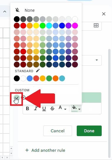
– Click on the Color you want to fill the cell with
– Here we selected green
Step 7 – Click on the Done option
– After selecting the color, click on Done
Step 8 – Copy the Formatting
– After getting the result in the cell, drag the cell down till the desired cell of that column to apply the same formatting in the column


