How to count checkboxes in Google Sheets

In Google Sheets, checkboxes are a type of data validation that allows users to select or deselect a binary choice. They are represented by small square boxes that can be checked or unchecked by clicking on them. Checkboxes are commonly used in spreadsheets to track tasks, mark completion status, or create interactive forms.

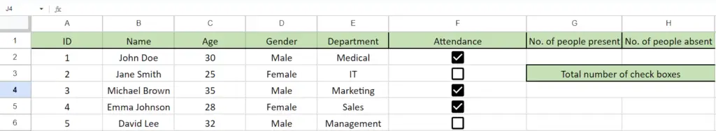
The dataset provides basic information about employees, including their unique identifiers, names, ages, genders, the departments they belong to, and their attendance in the form of checkboxes. In today’s tutorial, we will learn how to count the ticked, unticked, and total number of checkboxes.

Case 1 – Counting the ticked check-boxes

Step 1 – Selecting the cell

• Firstly, select any cell in which you want to calculate the number of ticked checkboxes.
• In this cell, we will apply the COUNTIF Formula to get the total number of ticked checkboxes.

Step 2 – Writing the formula

• In the selected cell type “=” (without quotes) and then write COUNTIF in the selected cell and select the COUNTIF Function by pressing the tab button on your keyboard.
• Then, select the range of cells in which the checkboxes are present. For example, we’ve selected the range of cells (F2:F6).
• After doing that, press the comma (,) button on your keyboard and then write TRUE.
• Now, your formula would look like this,

=COUNTIF(F2:F6,TRUE)

Step 3 – Implementing the formula

• Then, close the parenthesis and press Enter.
• After that, the result would appear on the screen which is 3, and as you can see the 3 checkboxes are ticked and the answer is according to it.

Case 2 – Counting the unticked checkboxes

Step 1 – Selecting the cell

• First of all, select any vacant cell in which you want to calculate the number of unticked checkboxes.
• In this cell, we will use the COUNTIF Formula in this cell to get the total number of unticked checkboxes.

Step 2 – Writing the formula

• Type “=” (without quotes) in the selected cell, followed by “COUNTIF”.
• Press the Tab button on your keyboard to select the COUNTIF Function.
• Select the range of cells where the checkboxes are located. For example, if the checkboxes are in cells F2 to F6, select that range.
• Press the comma (,) button on your keyboard.
• Type “FALSE” (without quotes) after the comma.
• Your formula should now look like this:

=COUNTIF(F2:F6, FALSE)

Step 3 – Implementing the formula

• Close the parenthesis and press Enter.
• The result will appear on the screen, indicating the number of unticked checkboxes. For example, if the result is 2, it means that 2 checkboxes are unticked.

Case 3 – Counting the ticked and unticked checkboxes

Step 1 – Selecting the cell

• First of all, select any vacant cell in which you want to calculate the total number of checkboxes.
• In this cell, we will use the SUM Function to find the total number of checkboxes.

Step 2 – Writing the formula

• Firstly, write = (equal sign) in the selected cell.
• Then, type SUM and select the SUM Function by using the tab button on your keyboard.
• After that, select or enter the name of the cell in which the result of the total ticked checkboxes is present. For example, it is cell G2 in our case.
• Then, press the comma (,) button and then select or enter the name of the cell in which the result of total unticked checkboxes is present. For example, it is cell H2 in our case.
• Now your formula would look like this,

=SUM(G2,H2)

Step 3 – Implementing the formula

• After writing the formula, close the parenthesis and press Enter.
• The result would appear in the cell which is 5 and as we can see the total number of checkboxes is 5 which is according to the answer.