How To Use Checkboxes In Google Sheets

In this tutorial we are going to learn how to add and then use the checkboxes (tick boxes) in Google sheets. Google Sheets has termed Check boxes as “Tick boxes” so we will use the term which is used by Google Sheets to avoid any confusions.

Let’s take an example of daily tasks lists and explore how tick boxes can help us to track the current status of our daily tasks. Following is the Google Sheet with some tasks in it.

Google is making developments and adding more and more features to Google Sheets to make it more compatible with Excel Spreadsheets. One such feature is the ability to add “Checkboxes” or “Tick boxes” in Google Sheets.

Step 1 – Add Tick Boxes to the desired column

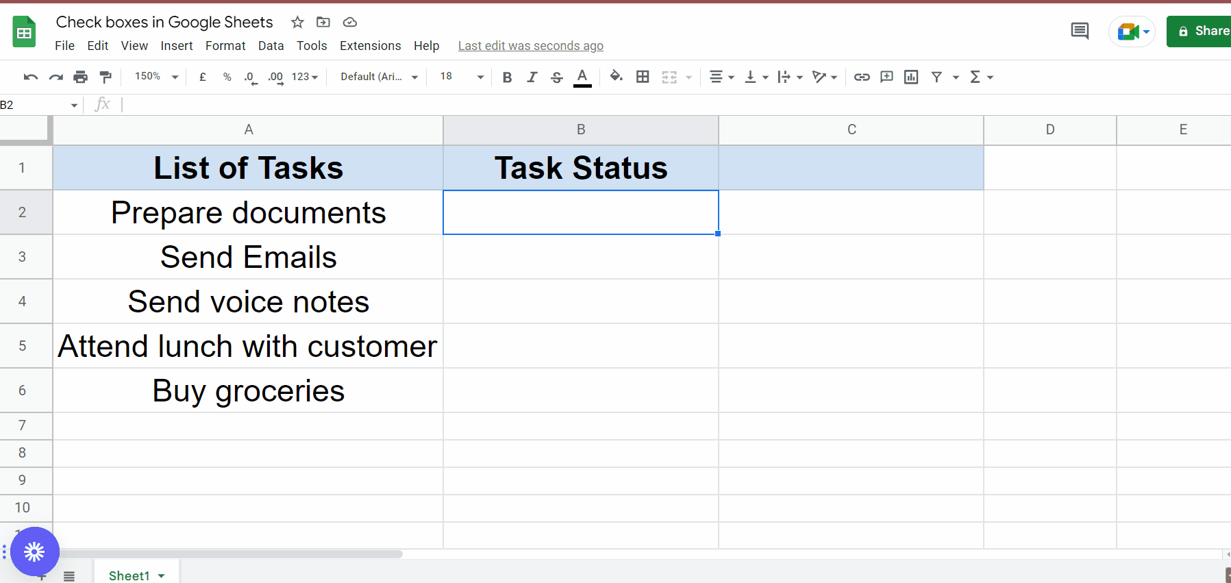
– To add tick boxes in google sheets, first select all those cells in which you wish to add the tick boxes.

– Then click on the Insert tab and locate the Tick box button. Click the button to add tick boxes in all the cells as shown in the figure above.

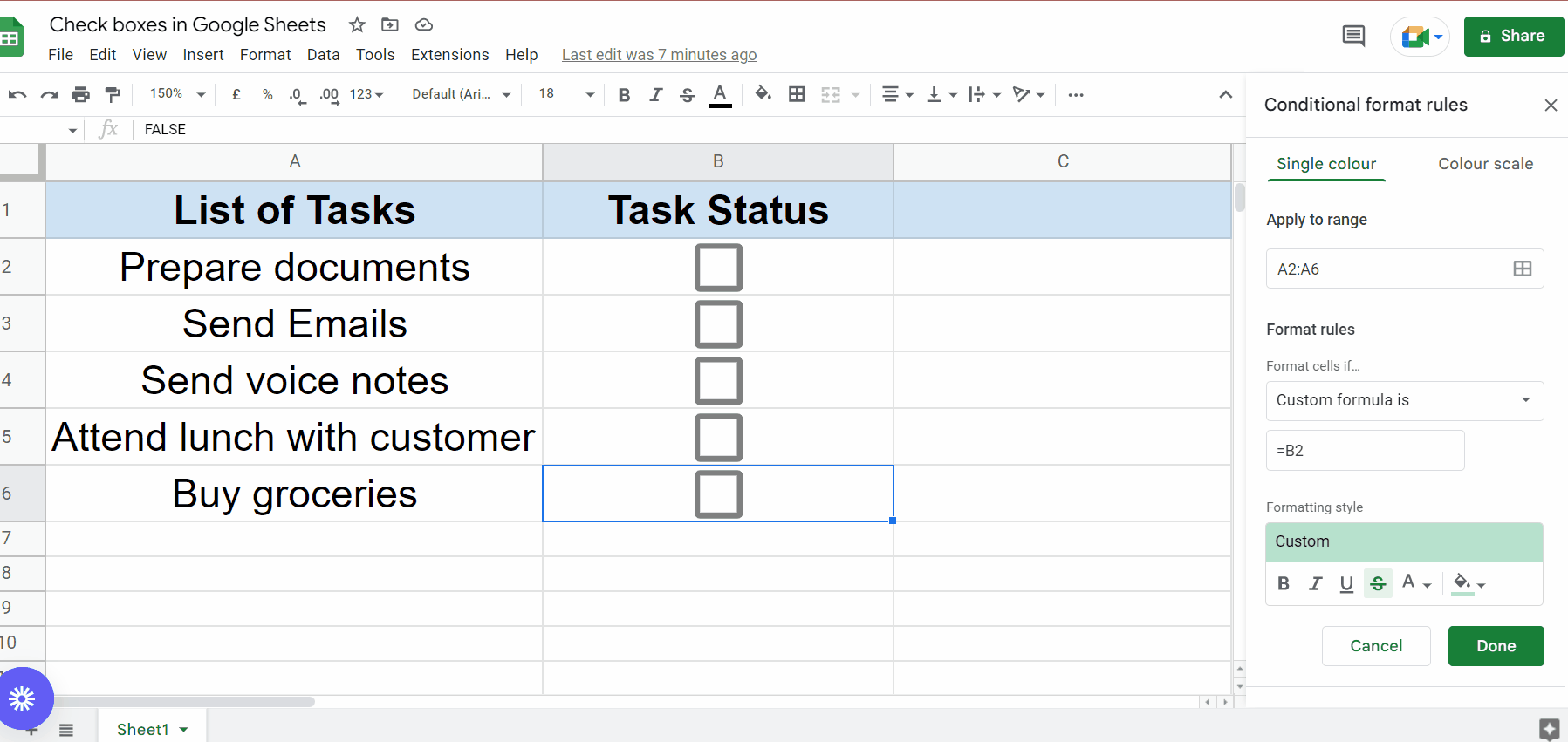
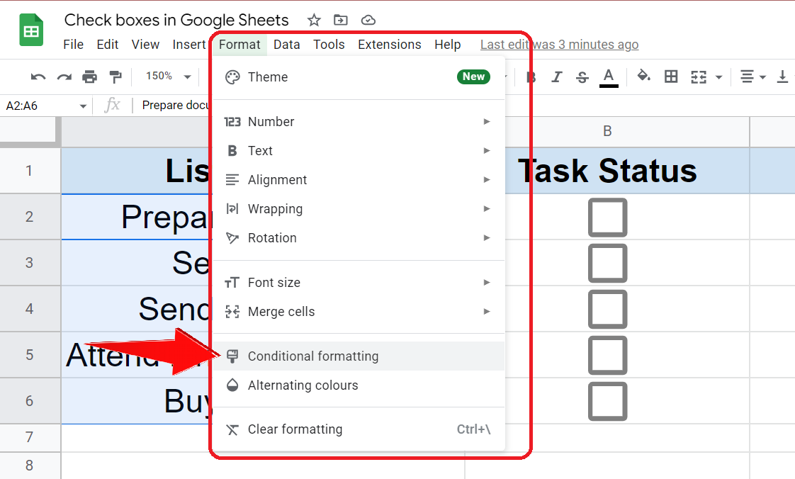
Step 2 – Select all the entries in tasks list and open conditional formatting

– Now we will use the conditional formatting’s “custom formula is” category to create an interactive checklist. For this purpose first select all the entries in the task list.

– Now click on the Format tab and select conditional formatting. Following window will open;

Step 3 – Create a custom formula for conditional formatting

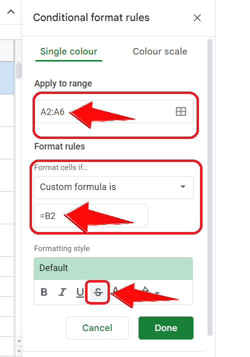
– A new sidebar will become visible with the name “Conditional format rules”. In there locate “format rule” and select “custom formula is”.

– Enter the following formula;
=B2

This formula tells Google Sheets to format all the respective cells, mentioned in the “apply to range” when any value in Column B starting from B2 becomes true. The process of applying the formula is shown in the figure above.