How to Make Every Other Row Shaded in Google Sheets
 By
SpreadCheaters
By
SpreadCheaters
Google Sheets is a widely used tool for organizing, analyzing, and visualizing data. Whether you’re a student, researcher, or working professional, Google Sheets can help you keep track of important information in an efficient manner. However, when dealing with large datasets, it can become difficult to read and differentiate between rows, which can lead to errors and confusion. One simple way to improve readability is by shading every other row. This technique not only makes your data easier to read but also adds a professional touch to your spreadsheets.
Thankfully, making every other row shaded in Google Sheets is an easy process that anyone can learn. By following a few simple steps, you can quickly alternate the row colours and create a visually appealing spreadsheet. In this article, we’ll walk you through the process of shading every other row in Google Sheets, so you can make your data more organized and professional.
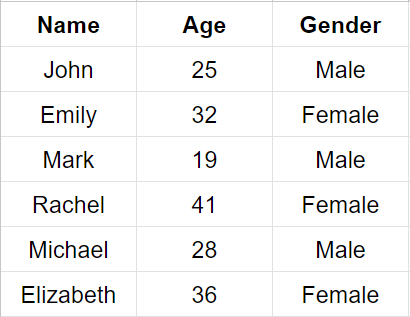
So, let’s dive into the steps to make every other row shaded in Google Sheets with the help of the following dataset.
Method 1 – Alternating Colours
Step 1 – Select Data

- Select your data.
Step 2 – Go To Format Menu
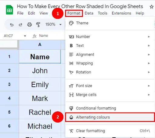
- Go to the Format menu & select Alternating Colours.
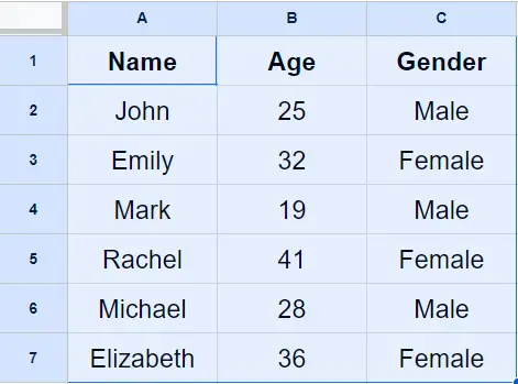
Step 3 – Alternating Colour Pane

- Alternating colour pane will be open at the right side of your screen.
- Choose any of the default styles, or you can make your own custom style. Mark check for Header and Footer.
- Click the DONE button when finished.
Method 2 – Conditional Formatting
Step 1 – Select Columns
- Select column range where you want to enter dynamic data. For our example, we will select column A to C.
Step 2 – Go To Format Menu
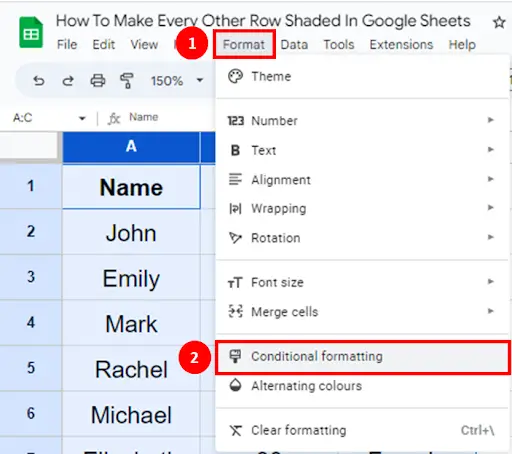
- Go to the Format menu & select Conditional Formatting.
Step 3 – Conditional Formatting Pane
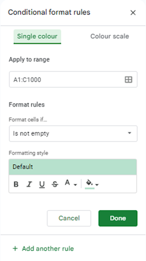
- Conditional Formatting Pane will appear at the right side of your screen.
Step 4 – Set Conditional Formatting Rule

- Notice that range is already applied as we had selected the columns in step 1.
- From the Format Rules drop down list, select Custom formula is.
- Type this formula: =AND(NOT(ISBLANK($A2)),ISODD(ROW())).
- Set formatting style & click on the DONE button.
- The beauty of this method is that it is a dynamic solution. The rows will be shaded automatically, when you add more data into your table.
Formula Breakdown
=AND(NOT(ISBLANK($A2)),ISODD(ROW()))
The formula is used to determine whether a cell meets certain conditions, and it returns a TRUE or FALSE value.
The formula contains two logical functions, NOT and AND, as well as two functions that test cell values, ISBLANK and ISODD.
Here’s what each function does:
- NOT(ISBLANK($A2)): This function tests whether cell A2 is empty or not. The ISBLANK function returns TRUE if the cell is blank, and the NOT function negates this result so that it returns FALSE if the cell is blank, and TRUE if it contains any value.
- ISODD(ROW()): This function tests whether the row number of the current cell is odd or even. The ROW function returns the row number of the current cell, and the ISODD function returns TRUE if the row number is odd, and FALSE if it’s even.
- AND(logical1, logical2): This function tests whether two logical expressions are both TRUE or not. In this case, the two expressions are the results of the previous two functions. The AND function returns TRUE only if both expressions are TRUE, and FALSE otherwise.
Therefore, the overall meaning of the formula is: “Return TRUE if the cell is not blank and the row number is odd. Otherwise, return FALSE.”