
How to find repeats in Google Sheets
 By
SpreadCheaters
By
SpreadCheaters
In Google Sheets, finding repeats means identifying and highlighting any duplicate values or entries within a specific range of cells or an entire sheet. This can be useful when working with large sets of data, as it can help you to quickly identify and remove any redundant or unnecessary information.
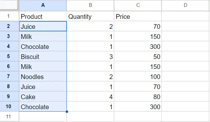
Our data set has a grocery store bill that includes the names, quantities, and prices of various products. Some of the products are repeated, and we want to identify them. To do this, we will use customized conditional formatting, which will utilize the COUNTIF function. Following steps will guide you to use the conditional formatting.
Method 1: Find Repeats in a Single Column
Step 1 – Select the Range of Cells

- Select the range of cells, from which you want to find the repeats
Step 2 – Click on the Format tab
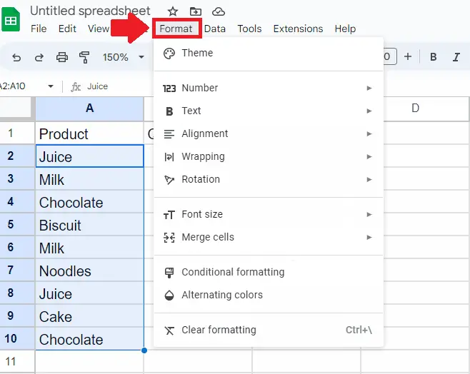
- After selecting the range of cells, click on the Format tab from the taskbar and a drop-down menu will appear
Step 3 – Click on the Conditional Formatting option
- In the drop-down menu, click on the Conditional Formatting option and a dialog box will appear on the right side of the sheet
Step 4 – Click on Custom Formula
- In the dialog box, click on the arrow next to the box below the Format rules option and a drop-down menu will appear
- From this menu, click on the Custom Formula option and a dialog box will appear
Step 5 – Type the Formula
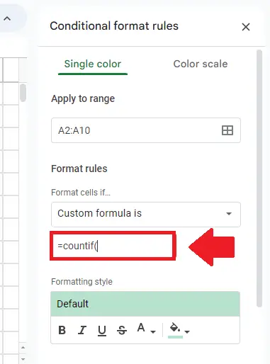
- In the dialog box, type the formula(in the box below the “custom formula is” box) below
- =Countif(
Step 6 – Type the Arguments
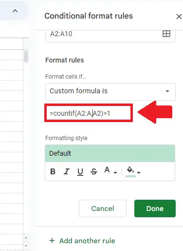
- After typing the formula, type its arguments:
- Starting cell: A2
- End Column: A
- Starting Cell: A2
- After typing the arguments, type the closing bracket along with a lesser than symbol “)>1”
Step 7 – Click on Done
- After typing the formula, click on Done to get the result
Method 2 Find Repeats across multiple columns and rows
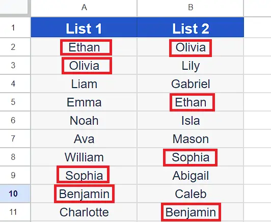
Sometimes, the duplicate entries are found in other columns and rows as well. In that case the formula for conditional formatting will have to be changed accordingly. Let’s see how to do this by following the steps mentioned below. We have a dataset above of two list of names and we wish to find and highlight the duplicate names only. As we can see that there are four duplicate names in the lists.
Step 1 – Select the range of cells
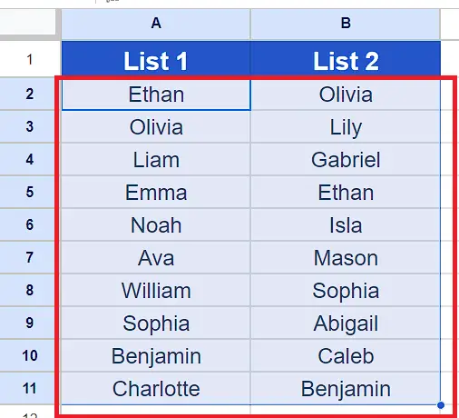
- Select all cells of the range from which you wish to find and highlight the duplicates as shown above.
Step 2 – Click on the Format tab
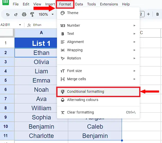
- After selecting the range of cells, click on the Format tab from the taskbar and a drop-down menu will appear.
- From this drop-down menu click on the Conditional Formatting option.
Step 3 – Choose Custom Formula Option in Format Rules
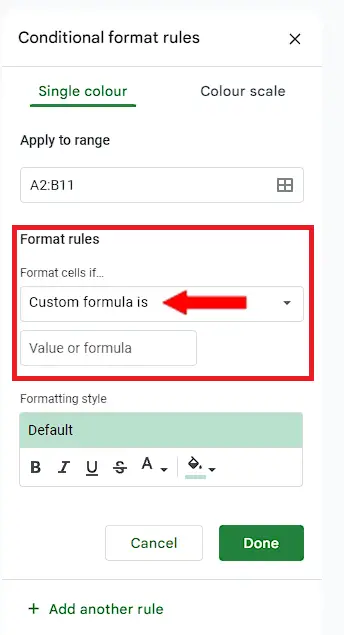
- From the newly opened Conditional Format Rules side bar, choose the Custom Formula option in Format Rules field, as shown above.
Step 4 – Write the following Custom Formula to highlight duplicates

- In Custom Formula Field write the following formula in Value of Formula option as shown above.
=COUNTIF($A$2:B11,Indirect(Address(Row(),Column(),)))>1
Step 5 – Choose the formatting style and press Done
- In the formatting style Field choose whatever color or fonts you want to use for highlighting the duplicates. In our case, we’ll use the default highlighting only.
- Now press the Done button and all the duplicates will be highlighted as shown above.
Breakdown of the formula
=COUNTIF($A$2:B11,Indirect(Address(Row(),Column(),)))>1
This formula is used in conditional formatting rules in Google Sheets to highlight duplicates in a range of cells.
Here is a breakdown of how it works:
COUNTIF: This function counts the number of times a specified value appears in a range of cells.
$A$2:B11: This is the range of cells that you want to check for duplicates. The first cell in the range is locked with the $ sign to make sure that it does not change when the formula is applied to other cells.
Indirect(Address(Row(),Column(),)): This returns the address of the current cell, which is then used as a reference to check for duplicates.
>1: This part of the formula checks whether the count of the current cell’s value in the specified range is greater than 1. If it is, the cell is considered a duplicate and the conditional formatting rule is applied to highlight it.
So when this formula is applied as a conditional formatting rule in Google Sheets, it checks each cell in the specified range to see if it appears more than once. If it does, the cell is highlighted as a duplicate.


