
How to do cumulative sum in Excel
 By
SpreadCheaters
By
SpreadCheaters
Cumulative sum in Excel is a mathematical operation that calculates the total sum of a series of values over time such as a sequence of months or years. It represents the sum of all the previous numbers in the series, including the current value. You can use the cumulative sum in Excel to analyse data trends and track progress over time, such as cumulative revenue, cumulative expenses, or cumulative profits.
Method 1 – Using Sum Function
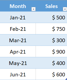
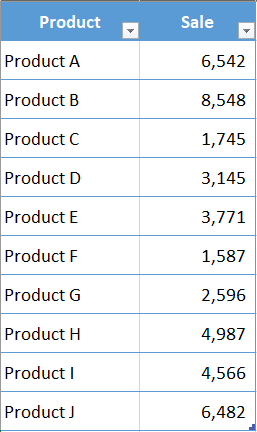
In this tutorial, we’ll learn how to calculate the cumulative sum or total in Excel. Let’s understand with an example. Suppose that we have the following sales data for six months & we want to find out cumulative sales for these months.
Step 1 – Add New Column
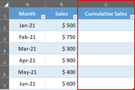
- Add a new column to your table & name it as “Cumulative Sales”. In our example, it’s column C.
Step 2 – Type Formula
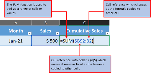
- In cell C2 type the following formula.
- We will press the F4 button to place a dollar sign to fix the cell reference.
Step 3 – Drag The Formula
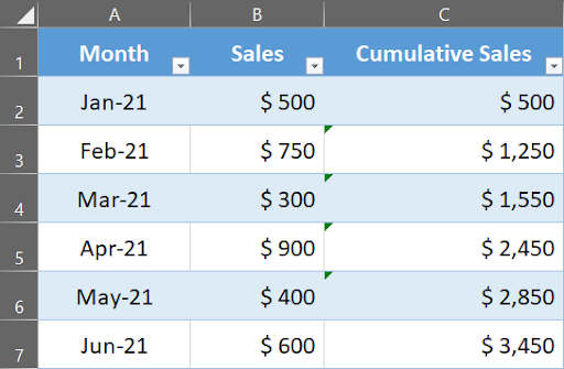
- Drag the formula down to apply it to the remaining cells in the column.
Step 4 – Cumulative Sum Calculated
- Cumulative sales of the data is calculated.
Method 2 – Calculating Running Total Using Power Query
Power Query is an amazing tool when it comes to connecting with databases, extracting the data from multiple sources, and transforming it before putting it into Excel.
If you are already working with Power Query, it would be more efficient to add running totals while you are transforming the data within the Power Query editor itself (instead of 1st getting the data in Excel and then adding the running totals using any of the method covered above).
While there is no inbuilt feature in Power Query to add running totals (which I wish there was), you can still do that using a simple formula.
Suppose you have an Excel table as shown above and you want to add the running totals to this data:
Step 1 – Select Data Tab
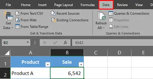
- Click any cell in the Excel Table.
- Click on Data Tab.
Step 2 – Click From Table / Range Button
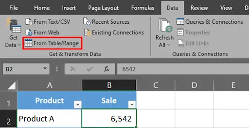
- In the Get & Transform Data group click From Table / Range button.
- Power query editor will open on your screen.
Step 3 – Click Add Column
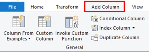
- In the power query editor, click on Add column tab.
Step 4 – Click Index Column Drop Down Button
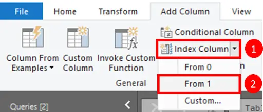
- In the General group, click on the index column drop down button.
- Click From 1 option. Doing this will add a new index column that would start from 01 and enter the numbers incrementing by 1 in the entire column.
Step 5 – Index Column Inserted
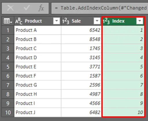
- This will add an index column in your editor screen.
Step 6 – Click On The Custom Column Button
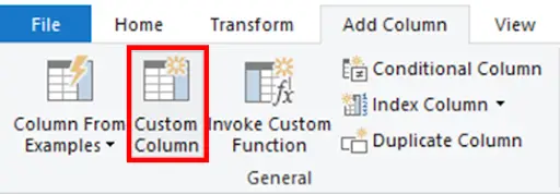
- Now click on the custom column button.
Step 7 – Type Column Name
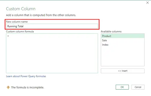
- Type column name in the custom column dialog box that appears on your screen.
Step 8 – Type The Formula
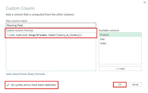
- In the custom column formula field, enter the following formula.
- Make sure that there is a checkbox at the bottom of the dialog box that says “No syntax errors have been detected.
- Click OK button.
Step 9 – Running Total Column Added
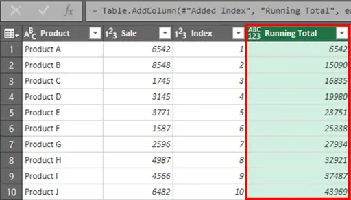
- Running Total Column will be inserted in the power query editor screen.
Step 10 – Remove Index Column
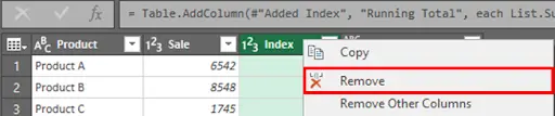
- Right click on the index column & remove it.
Step 11 – Click On The File Tab
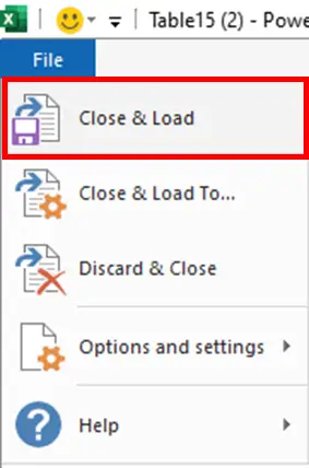
- Click on the File tab & select close & load option.
Step 12 – New Worksheet Inserted
- This would insert a new worksheet in your workbook with a table that has the running totals.
Breaking Down The Power Query Formula
List.Sum(List.Range(#”Added Index”[Sale],0,[Index]))
- The first thing we do in the Power Query editor is to insert an index column starting from one and incrementing by one as it goes down the cells.
- We do this because we need to use this column while we calculate the running total in another column that we insert in the next step.
- Then we insert a custom column and use the below formula
- List.Sum(List.Range(#”Added Index”[Sale],0,[Index]))
- This is a List.Sum formula that would give you the sum of the range that is specified within it.
- And that range is specified using the List.Range function.
- The List.Range function gives the specified range in the sale column as the output and this range changes based on the Index value. For example, for the first record, the range would simply be the first sale value. And as you go down the cells, this range would expand.
- So, for the first cell. List.Sum would only give you the sum of the first sale value, and for the second cell, it would give you the sum for the first two sale values and so on.


