How to keep a Running Balance in Excel

A running balance is the current total balance of an account, which takes into account all previous transactions as well as any subsequent deposits or withdrawals. A running balance is a useful tool for tracking spending and managing finances, as it provides a real-time snapshot of the account balance. It is commonly used in bank statements, financial statements, and accounting software, allowing users to monitor their account activity and balance over time. By keeping track of the running balance, users can identify any discrepancies, monitor their spending, and ensure they have enough funds available for future expenses.

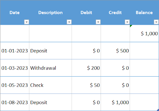
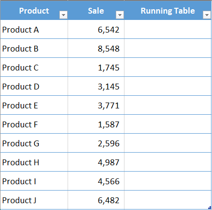
Now, let’s understand it with the following methods. Suppose we have the following dataset shown above & want to calculate the running balance of a bank account.

Understanding The Formula

Before moving on, let’s understand the formula first. To calculate the running balance will be using the following formula.

=Previous balance + Credit Amount – Debit Amount

The formula is quite simple. We will add credit amounts to the previous balance & subtract the debit amounts. Now let’s apply it in our example.

Method 1 – Manual Calculation With Cell Reference

Step 1 –  Place Equals To Sign

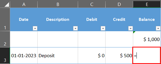
• Start typing the formula by placing equals to sign (=).

Step 2 – Type The Formula

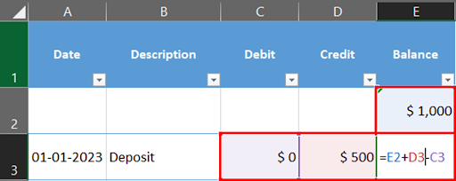
• Type the formula.

Step 3 – Drag The Formula Downwards

• Press enter.
• Drag the formula downwards to the remaining cells using selection handle.

Method 2 – Calculating Running Total With Excel Table

The most effective way to work with tabular data is to convert it into an Excel table. It makes managing data easier, as well as making tools like Power Query and Power Pivot easier to use.

The use of Excel tables comes with a variety of advantages, including structured references, automatic reference adjustment, and easy access to data in the table for formulae.

Suppose you have an Excel table as shown above and you want to calculate the running total in column C.

Step 1 –  Place Equals To Sign

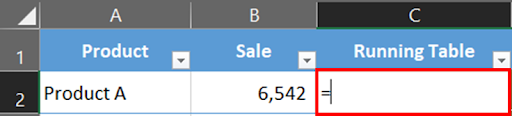
• Start typing the formula by placing equals to sign (=).

Step 2 –  Type The Formula

• In column C, start typing the formula. We will break it down later.

Step 3 – Running Total Calculated

• Press enter.
• The formula will be applied automatically to all the remaining cells down above.

Breaking Down The Above Formula

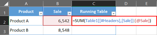
=SUM(Table1[[#Headers],[Sale]]:[@Sale])

The above formula may look a bit long, but you don’t have to write it yourself. What you see within the sum formula are called structured references, which is Excel’s efficient way to refer to specific data points in an Excel table. For example, Table1[[#Headers],[Sale]] refers to the Sale header in Table 1 (in other words, cell B1) And [@Sale] refers to the value in the cell in the same row in the Sale column (cell B2).

You will also notice that you don’t have to copy the formula in the entire column, an Excel table automatically does it for you.

Another great thing about this method is that in case you add a new record in this data set, the Excel table would automatically calculates the running total for all the new records.

While we have included the header of the column in our formula, remember that the formula would ignore the header text and only consider the data in the column.