How to use Pi in Google Sheets

In mathematics, π (pi) is a mathematical constant that represents the ratio of the circumference of a circle to its diameter. It is an irrational number, which means it cannot be expressed as a simple fraction and its decimal representation goes on forever without repeating. The value of π is approximately 3.14159, but it is often approximated as 3.14 for simplicity in calculations. In Excel, there is a specific function of Pi to calculate values.

In this Excel tutorial, we will explore the functionality of the “PI” function, which allows us to calculate the circumference of a circle. Additionally, we will discover how to insert the π (pi) symbol as text within cells. By mastering these techniques, you will gain valuable skills in utilizing mathematical constants and enhancing your Excel spreadsheets with precise calculations and visual representations.

Case 1 – Using the “PI” Function to calculate the circumference

Understanding Function and its Syntax

The “PI” function in Excel is a built-in mathematical function that returns the value of π (pi), which is approximately 3.14159. 

The syntax of the “PI” function is as follows:

=PI()

The function does not require any arguments or parameters, so you simply use the function name followed by opening and closing parentheses. When the function is used in a cell, it will automatically return the value of π. This value can then be used in mathematical calculations within Excel, such as calculating the circumference or area of a circle.

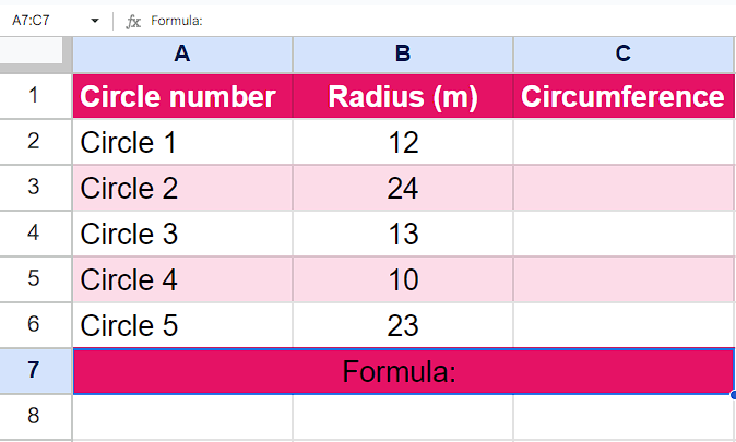
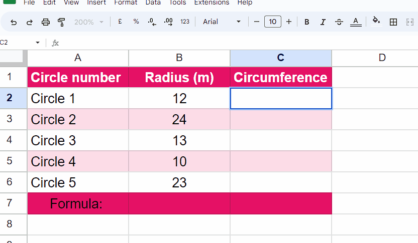
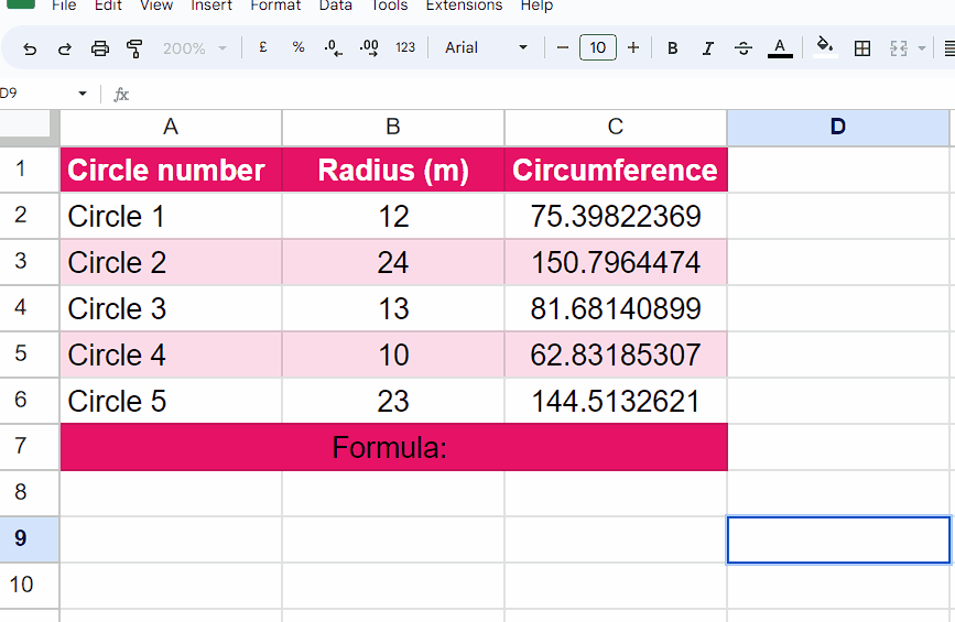
Step 1 – Select the cell

• Select any empty cell in which you wish to find the circumference of the circle
• We will use the “PI” Function in this cell to get our desired results.

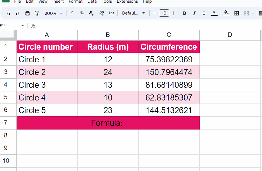
Step 2 – Write the formula and implement it

• In the chosen cell, start by entering the equal sign (=) to initiate the formula.
• Next, type “2*PI()” to incorporate the 2 multiplied by the value of π (pi) into the formula.
• Following that, insert an asterisk () to indicate multiplication.
• Then, specify the cell reference B2 as the value that will be multiplied by 2π.
• Now that you have followed all the steps above, your formula would look like this,

=2*PI()*B2)

• Then, press Enter and your answer would appear.
• If you want to implement the formula to the whole range then click on the “tick ✔” option of the Auto-fill.

Case 2 – Inserting the “PI (π)” symbol

Step 1 – Select the cell

• Select any empty cell in which you can apply the “CHAR” function to get the “PI (π)” symbol.

Step 2 – Write the formula

• After selecting the cell, write the following formula in the cell

=CHAR(960)

• It will give you the result as a “π” symbol.

Step 3 – Paste the “π” as Plain text

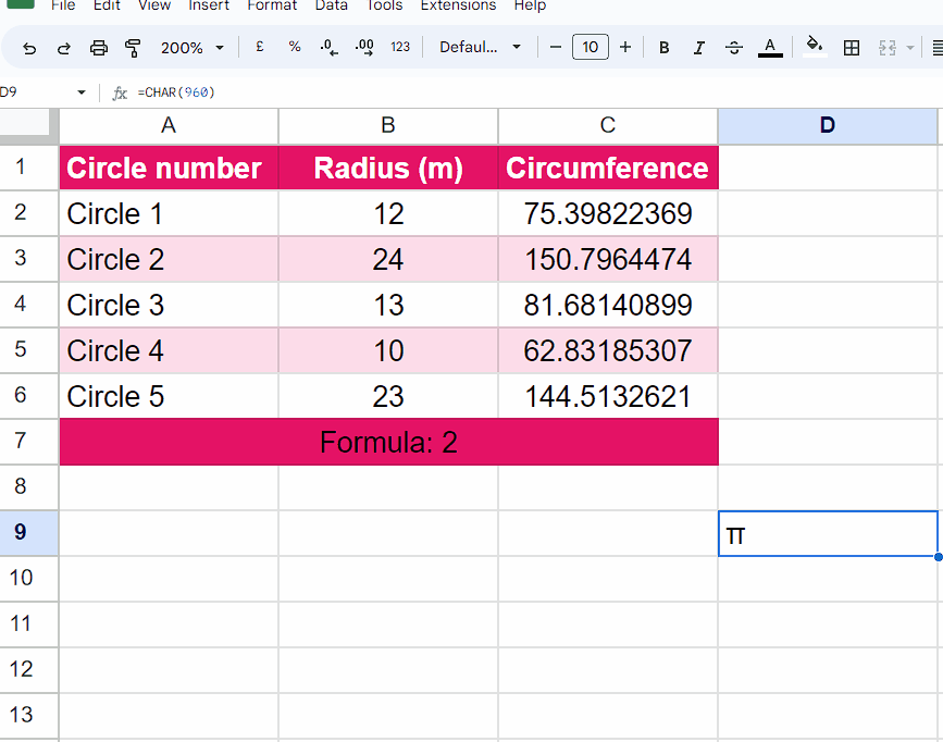
• After we get the “π” symbol, copy it because we want to paste it as text, not a formula.
• While writing the text where you want to insert it, right-click there and click on “Paste as Plain text” or use the shortcut key “Ctrl+Shift+V” to paste it as text.