How to paste horizontal data vertically in Google Sheets

There can be various reasons why we might need to transpose or paste horizontal data vertically in Google Sheets Sometimes, we may have data that is originally arranged horizontally, but we need it to be vertically aligned for analysis or presentation purposes. Transposing the data allows us to reorient it to a more suitable format.

There can be different ways to paste horizontal data vertically in google sheets. Two easy and simple ways to do this will be discussed in this tutorial. One way is to paste the horizontal data using the “Paste Special” option. Another way is to use the TRANSPOSE function.

Method 1 – Using Paste Special

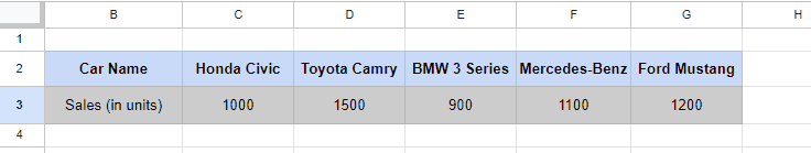
We can paste horizontal data vertically in google sheets by using the “paste special” option. While pasting the data, we’ll tickmark the transposed option. Consider the following dataset that contains sales of five different cars and their names arranged horizontally. We’ll copy and then paste the data vertically for better understanding.

Step 1 – Copy the data to be transposed

• Go to the location of the data that you want to transpose.
• Press and drag the cursor over the data, and then release it to select it.
• Right-click on data and click copy.
• Or simply press Ctrl+C to copy the data.

Step 2 – Paste the data using Paste Special

• Go to the location where you want to paste the data.
• Select a cell.
• Right-click on it,
• Click on Paste Special.
• Click on Transposed.
• The data will be pasted vertically.

Method 2 – Using the TRANSPOSE function

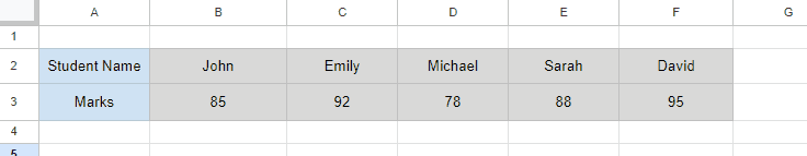
We can also use the TRANSPOSE function to paste horizontal data vertically in google sheets. This function changes the rows of the data into columns and vice versa. The difference, in this case, is that when we use the TRANSPOSE function, the formatting is not copied to the transposed data. Consider the data that contains the marks of five students:

Step 1 – Select the cell where you want to paste the data vertically

• Go to the location where you want to paste the data.
• Click on the cell to select it.

Step 2 – Use the TRANSPOSE function

• Write the appropriate formula using the TRANSPOSE function and the cell range that contains the horizontal data in the selected cell.
• In this case, the formula is =TRANSPOSE(A2:F3), where A2:F3 is the cell range that has the horizontal data.
• Press Enter.