
How to make horizontal data vertical in Excel
 By
SpreadCheaters
By
SpreadCheaters
To make horizontal data vertical in Excel means to transform data that is arranged in rows horizontally into a vertical orientation. By making the data vertical, we can more easily analyze and manipulate the data in Excel, and it can be easier to present the data in a more readable format.
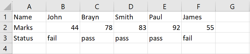
The results of the students in our dataset, which include their names, marks, and status, are currently displayed horizontally. However, we want to display this data vertically. We have two options to achieve this: The first method involves. The first method is by pasting the transpose and the second method is by using the Transpose option. These methods are explained in the following steps.
Method 1: Transpose data using the paste option
Step 1 – Select the Range of Data
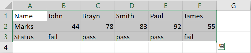
- Select the range of cells to be flipped by using drag and drop method
Step 2 – Open the Context menu
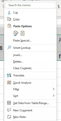
- Right-click anywhere in the selected range of cells to open the context menu
Step 3 – Copy the Data
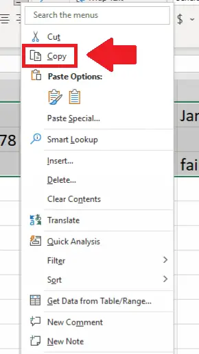
- In the context menu, click on the Copy option
Step 4 – Select the Cell
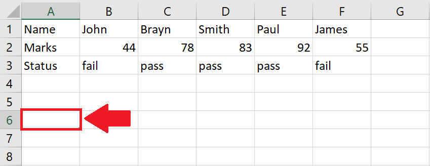
- Click on the cell where you want to show the flipped data
Step 5 – Open the Context menu
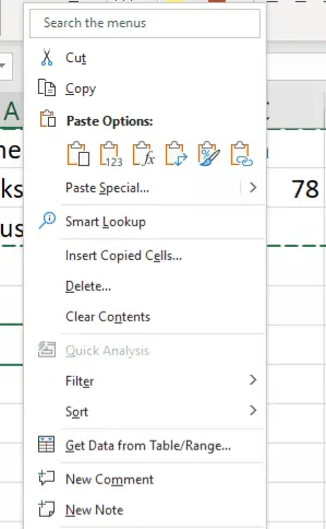
- Right-click in the selected cell to open the context menu
Step 6 – Click on Transpose

- In the context menu, click on the Transpose option in the list above the Paste option
Method 2: Transpose data using the Transpose function
The Excel TRANSPOSE function “flips” the orientation of a given range or array: TRANSPOSE flips a vertical range to a horizontal range and flips a horizontal range to a vertical range.
Syntax of the Transpose function is:
=TRANSPOSE(array)
- The array argument is a range of cells to be flipped.
Step 1 – Select the cell
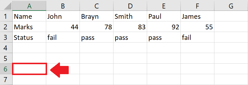
- Click on the cell, where you want to show the vertical data
Step 2 – Use the Transpose function
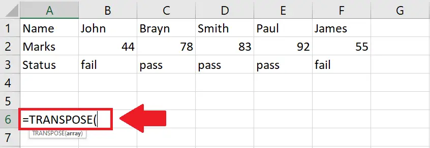
- To use the transpose function, type “=Transpose(” in the selected cell
Step 3 – Type the Argument of the function
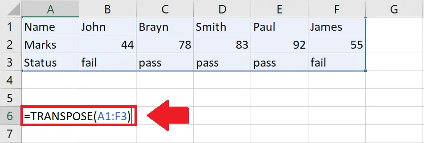
- Type the argument of the Transpose function(array)
- array: A1:F3
- After typing the argument, type the closing bracket “)”
Step 4 – Press the Enter key

- After typing the argument, press the Enter key to get the required result


