
How to leave a cell blank if false
 By
SpreadCheaters
By
SpreadCheaters
In Excel, leaving a cell blank if false refers to setting the value of a cell to empty or blank when a specific condition is evaluated as false. This can be achieved using Excel’s IF function or conditional formatting.
In this tutorial, we will learn how to leave a cell blank if false. Leaving a cell blank if a certain condition is false is a very simple task that a user can achieve by utilizing the IF function, the Find and Replace command, or the SUBSTITUTE function.
We currently have a dataset that includes student names, grades, and remarks. Our objective is to identify the students who have received an A grade and leave the cells blank for those who did not achieve an A grade.
Method 1: Utilizing the IF Function
To leave a cell blank in Excel when a condition is false, one of the most common and straightforward approaches is to utilize the IF function. In this case, you would set the “value_if_false” parameter of the IF function as an empty value, represented by two quotation marks (“”).
Step 1 – Apply the IF Function and Input the Condition and the “value_if_true”
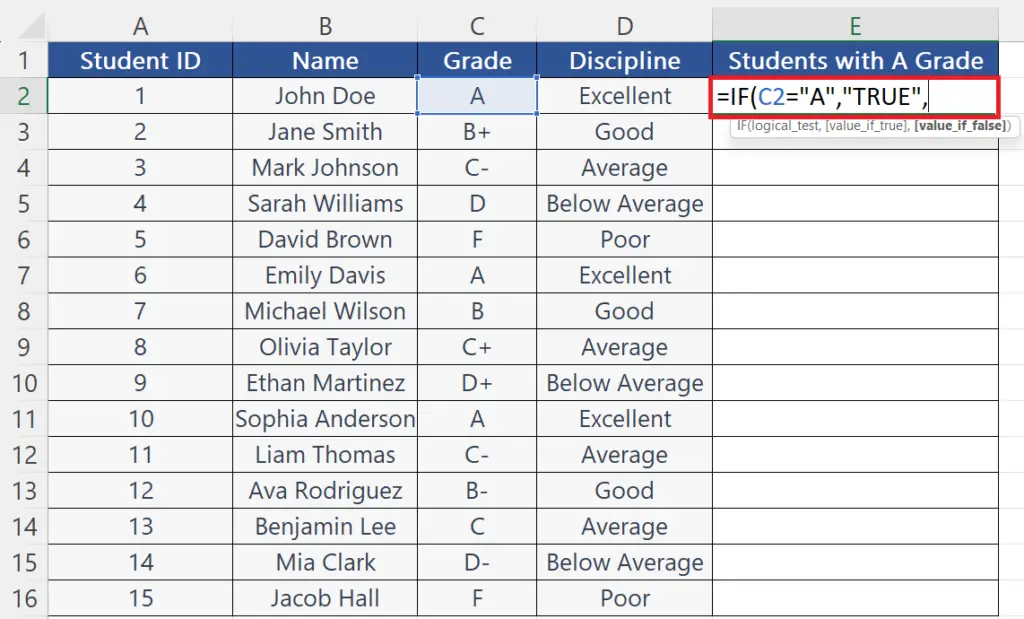
- Apply the IF function in an empty cell.
- Input the condition i.e. the logical test on the basis of which you want to evaluate.
- Input the “value_if_true” as required in this case we will input “TRUE”.
IF(C2= ”A”, “TRUE”.
Step 2 – Enter a Blank Value as “value_if_false”
- Enter a blank value as “value_if_false”.
IF(C2= “A”,” TRUE”, “”)
Step 3 – Utilize Autofill
- Utilize autofill to apply the function on each cell.
Method 2: Leaving the Cell Blank if False utilizing the SUBSTITUTE Function
If we have already evaluated whether the condition is true or false and now we want to make the cell with “FALSE” blank, we can utilize the SUBSTITUTE function.
Step 1 – Apply the SUBSTITUTE Function
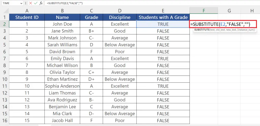
- Choose a blank cell to apply the substitute function.
- Enter the SUBSTITUTE function:
SUBSTITUTE(A2,”FALSE”, “”)
- Where A2 is the cell containing the value.
- “FALSE” is the text we want to replace.
- “” is a blank value i.e. the value which we want to substitute instead of “FALSE”.
Step 2 – Utilize Autofill to Apply the Function on Each Cell
- Utilize autofill to apply the function on each cell.
Step 3 – Paste the New Column on the Pre-Existing Column as Values
- Choose the column in which you have applied the SUBSTITUTE function.
- Hover the cursor on the border of the selection.
- Press hold the right mouse button and drag the column over the pre-existing column.
- Now drop the cursor, and a menu will appear.
- Choose the “Copy Here as Values Only” option.
Step 4 – Delete the New Column
- Now delete the column in which you have applied the SUBSTITUTE function.
Method 3: Utilizing the Find and Replace Command
If we have already evaluated whether the condition is true or false and now we want to make the cell with “FALSE” blank. Then we can also use another quick method i.e. the “Find and Replace” command. Following are the steps to utilize the “Find and Replace” command for this purpose.
Step 1 – Press the CTRL+H Keys
- Press the CTRL+H keys.
- This will open the “Find and Replace” dialog box.
Step 2 – Input “FALSE” in the “Find what” Field and Leave “Replace with” Feild
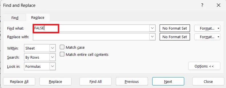
- Input “FALSE” in the “Find what” field.
- Leave the “Replace with” field empty.
Step 3 – Perform a Click on the “Replace All” Button
- Perform click on the “Replace All” button.
- The cells evaluated as “False” would become blank.


