
How to create a nested formula using average and round
 By
SpreadCheaters
By
SpreadCheaters
Page last updated:
28/06/2023 |
Next review date:
28/06/2025
A nested formula is used as an argument or component within another formula. In other words, it involves using one formula inside another formula to perform complex calculations or manipulate data in a more advanced way. Nested formulas allow you to perform sophisticated calculations by combining multiple functions and operations.
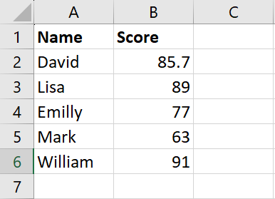
In this tutorial, we have demonstrated how to create a nested formula using the average and round functions. To create this we have four methods. The dataset consists of two columns, one for names and the other for scores. By utilizing nested formulas, we can perform advanced calculations and manipulate the score data in a more sophisticated manner.
Method 1: Use the Average first and then Round Function to create a nested formula
Step 1 – Type Average

- First, type Average in cell A8
Step 2 – Utilize Round and Average Function

- Now type Formula “=Round(Average(B2:B6),2) ”in cell B8 to find the first Average and then Round the result.
- “Average(B2:B6)” calculates the average of the values in cells B2 to B6.
- “Round(…,2)” takes the result of the average calculation and rounds it to two decimal places.
Step 3 – Press Enter Key
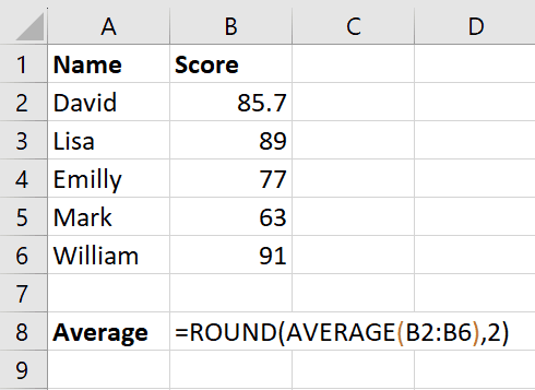
- Afterward, press Enter key and get the result
Method 2: Using the first Round and then Average Function to create a Nested Formula
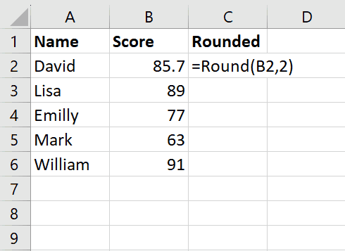
Step 1 – Create the Column with Header Name Rounded
- Now type Rounded in cell C1. This will be the column where we’ll get the rounded data.
Step 2 – Utilize Round Function
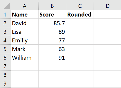
- Afterward, type Formula “=Round(B2,2)” in cell C2 to round off the values.
- “Round(B2,2)” takes the value in cell B2 and rounds it to two decimal places.
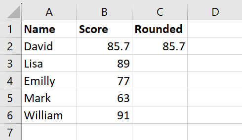
Step 3 – Press Enter Key
- After typing Formula press Enter key and get the Rounded values.
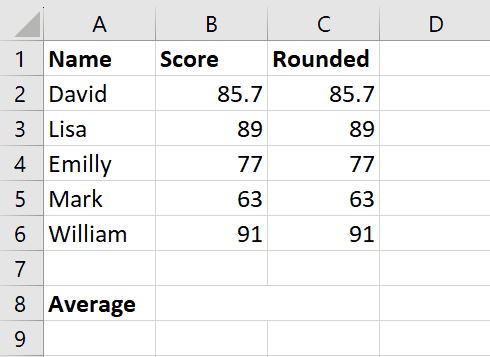
Step 4 – Drag the Formula
- Now drag the formula by clicking on the right corner of cell C2 it will give you the Round of all the Score.
Step 5 – Type Average
- After dragging the formula type Average in the cell A8
Step 6 – Utilize the Average Function
- Now type the Formula “=AVERAGE(C2:C6)”in cell B8 to find average
- “Average(C2:C6)” calculates the average of the values in cells C2 to C6
Step 7 – Press Enter Key
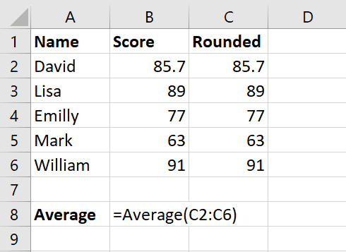
- After typing the Formula press Enter key and get the result


