
How to Calculate Weighted Average in Excel Pivot Table
 By
SpreadCheaters
By
SpreadCheaters
This is a step by step guide on how to calculate Weighted Average in an Excel Pivot Table.
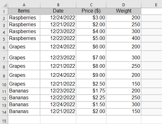
For example, we have a dataset containing different grocery items’ date-wise sales. Using a pivot table, we will calculate the weighted average price for each grocery item.

The weighted average is considered as the normal where not entirely settled for every amount expected to average. This sort of typical computation assists us with deciding the general significance of each sum by and large. A weighted normal can be viewed as more precise than any broad normal as every one of the numbers in the informational index are doled out to a similar weight.
Step 1 – Adding a new column
– First, in the table above, include a new column labeled “Sales Amount” as a “helper column.”. Next, enter the following formula into the first cell of this new column.
The syntax of this function is:
=(First Cell Address)*(Second Cell Address)
In our case it’s
=C2*D2
Step 2 – Copy The Formula to the Rest of the Columns
– You will now see the following results. Then, use the Fill Handle (+) tool to copy the formula to the rest of the column.
Step 3 – Select any cell within the data set
– To start building the pivot table, click on any cell within the dataset.
Step 4 – Insert Pivot Table
– Next, go to the Insert menu.
– Click on the Pivot Table option.
Step 5 – Select the Range
– A dialogue box will appear, select the range.
– Click on the ‘Ok’ Button.
Step 6 – Choose the Pivot Table Fields
– After that, the Pivot Table is created on a new sheet. Later, choose the PivotTable Fields as the below.
Step 7 – The Pivot Table will be created
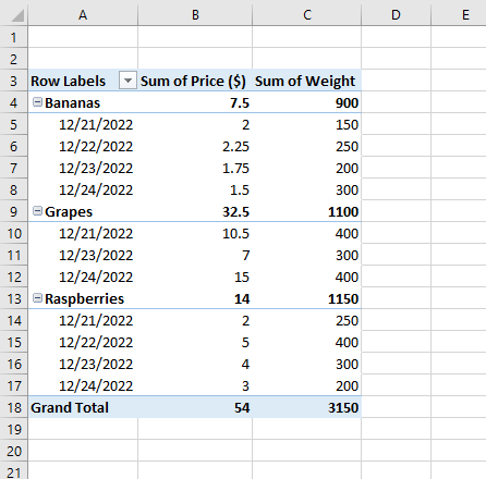
– The resulting Pivot Table is as follows.
Step 8 – Analyzing Weighted Average in Pivot Table
– Go to the Analyze tab.
– Select ‘Fields, Items, &Sets’ option.
– Add ‘Calculated Field’ from the given options.
Step 9 – Inserting the Calculated Field
– Now, type ‘Weighted Average’ on the Name field.
– Then, we have divided the helper column by weight (Sales Amount/Weight) to get the weighted average.
– Next, click on OK.
Step 10 – We obtained the Weighted Average
– Finally, In the subtotal rows of our pivot table, we obtained the weighted average price for each grocery item.
We tried to go into great detail about the weighted average calculation method in the above article. Also, this approach is very straightforward. You should be able to locate weighted averages in pivot tables with the help of the explanations.


