
How to calculate grade percentage in Excel
 By
SpreadCheaters
By
SpreadCheaters
Grade percentage is commonly used in Excel to calculate the grades of students or the performance of employees based on their performance on a test, exam, or project. Using grade percentages becomes an easy-to-understand way of evaluating how well someone has performed.
It also enables us to easily sort and filter data based on grade percentages. Grade percentages also help to automate the grading process, save time and reduce the likelihood of errors.
Grade percentages can be calculated in the following methods:
Method 1 – Make grades using vlookup
Grade percentage can be calculated using the Vlookup formula described in the following steps. In this method we will use Excel built-in function of VLOOKUP.
The syntax and description of vlookup is as follow;
=VLOOKUP(lookup_value, table_array, column_index_number, [range_lookup])
It consists of several components, each with its own purpose. Here’s a breakdown of the components:
Lookup value: This is the value you want to look up in the table. It can be a cell reference or a text string enclosed in double quotes.
Table array: This is the range of cells in which the lookup value will be searched. The table array must include the column containing the lookup value as well as the column containing the corresponding values you want to retrieve. The table array can also be a named range.
Column index number: This is the number of the column in the table array that contains the corresponding values you want to retrieve. The column index number starts with 1 for the first column in the table array, 2 for the second column, and so on.
Range lookup: This is an optional argument that specifies whether you want an exact match or an approximate match for the lookup value. If you want an exact match, set this argument to FALSE or 0. If you want an approximate match, set this argument to TRUE or 1. If you omit this argument, Excel assumes that you want an approximate match.
Step 1 – Make a table that contains the data
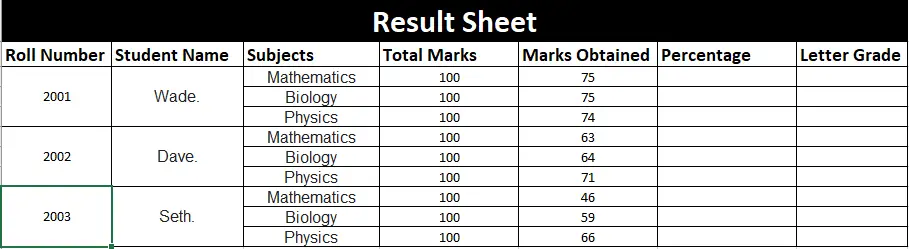
- Open the Excel worksheet.
- Make a table that shows what a person scored in an assignment.
- Enter the total number of points for the assignment. For example, if the assignment is worth 100 points, enter 100 in Total Marks.
- Enter the person’s score in the assignment in the Marks Obtained column.
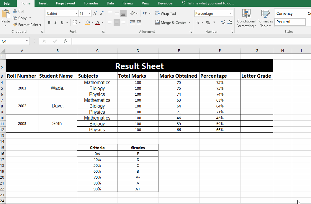
Step 2 – Calculate the Percentage
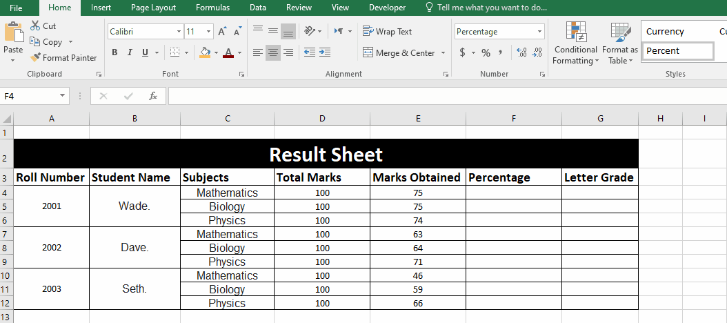
- In the percentage column, enter the formula to calculate the percentage. The formula is to divide the marks obtained by the total marks for the assignment and then multiply the result by 100%.
- Now drag down the formula to other cells to calculate percentages for other subjects and persons.
Step 3 – Make a table with the grade scale
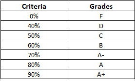
- Now to make grades by using Vlookup create a table with the grade scale and corresponding percentages. For example, if the grade scale is A+, A, A-, B, C, D, and F, and the corresponding percentages are 90%, 80%, 70%, 60%, 50%, 40%, and 0% respectively.
Step 4 – Use the Vlookup formula
- Select the cell where you want to look up the values. In this case, we selected cell G4.
- In this case we used this formula “=VLOOKUP(F4,$C$16:$D$22,2,TRUE)” to make grades in the next column. (Our lookup places are from C16 to D22).
- Now drag down the formula to other cells to calculate grade percentages for other subjects and persons.
- The process is shown in the animation below:
Method 2 – using nested IF
In this method, we can find grade percentages in excel by using the nested IF method.
We make comparisons of our percentages with our all grades given in the table as a reference.
The formula for grade percentages is as follow;
=IF(G2>=90%,$D$16,IF(G2>=80%,$D$17,IF(G2>=70%,$D$18,IF(G2>=60%,$D$19,$D$20))))
Firstly, It makes a comparison of our provided cell value with 90% , if it finds the value equal or greater, it will compare with cell value D16 which we have made absolute by adding a dollar sign. So that it only compares it with our $D$16.
Secondly, It makes a comparison of our provided cell value with 80% , if it finds the value equal or greater, it will compare with cell value D17 which we have made absolute by adding a dollar sign. So that it only compares it with our $D$17.
It will find and reflect till $D$20
The cell name shown in this formula will vary in your case. To find the grade percentages steps are given below;
Step 1 – Make a table with the grade scale
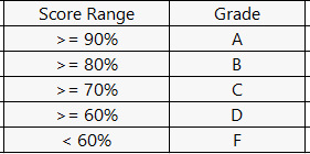
- Now to make grades by using Vlookup create a table with the grade scale and corresponding percentages. For example, if the grade scale is A, B, C, D, and F, and the corresponding percentages are 90%, 80%, 70%, 60%, respectively.
Step 2 – Select the desired cell
- Select the desired cell, where you wish to find grade percentages. In this case,we selected G2.
- Apply the formula in this case we have this formula
=IF(G2>=90%,$D$16,IF(G2>=80%,$D$17,IF(G2>=70%,$D$18,IF(G2>=60%,$D$19,$D$20))))
- As soon as you press the enter key, it will find and apply the grades among percentages.
- Fill other cells with the help of filler as shown below;
Hence, by using the above two methods we can find grade percentages in excel.


