Shortcut for Pivot Table in Microsoft Excel
A pivot table in Microsoft Excel is an effective data analysis tool that empowers users to organize and manipulate extensive data sets in a structured and interactive manner. It facilitates the extraction of valuable insights, trend analysis, and the formulation of data-driven conclusions.
In this article, we will discuss shortcuts for Pivot Table in Microsoft Excel. Utilizing keyboard shortcuts in Excel is a proficient approach to swiftly and effectively accomplish tasks.
Below we have listed some shortcuts that users can utilize while working with a pivot table in Excel.
Shortcut 1: Insert a Pivot Table
To, insert a pivot table in Excel, we need to perform multiple steps which is a time-consuming method. However, we can insert a pivot table instantly with the shortcut method.
Step 1 – Select the Range

- Select the range containing the data to insert a pivot table.
Step 2 – Press ALT+N+V+T Keys

- Press the ALT+N+V+T keys on the keyboard.
- Select where you want to insert the pivot table i.e. on the existing sheet or a new sheet.
- Click on OK, and the pivot table will be inserted.
Shortcut 2: Inserting a Pivot Table from the Pivot Table Wizard
We can also use the Pivot Table wizard to insert a pivot table. For this, below are the steps to be followed.
Step 1 – Select the Range
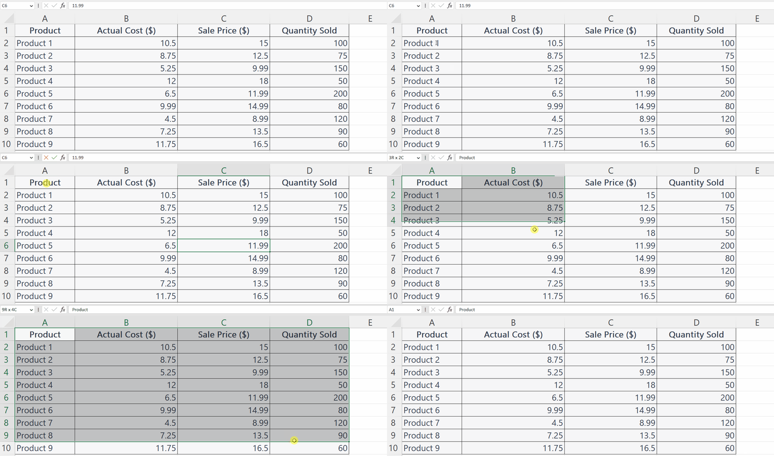
- Select the range containing the data to insert a pivot table.
Step 2 – Press ALT+D+P Keys
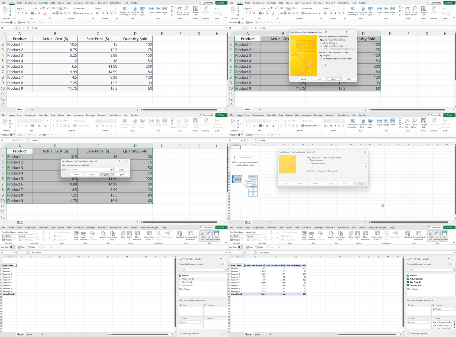
- Press the ALT+D+P keys on the keyboard.
- The pivot table wizard will appear.
- Insert the pivot table utilizing the wizard.
Shortcut 3: Create a Group
In a pivot table, grouping refers to the process of combining or categorizing specific items.
Step 1 – Select the Items
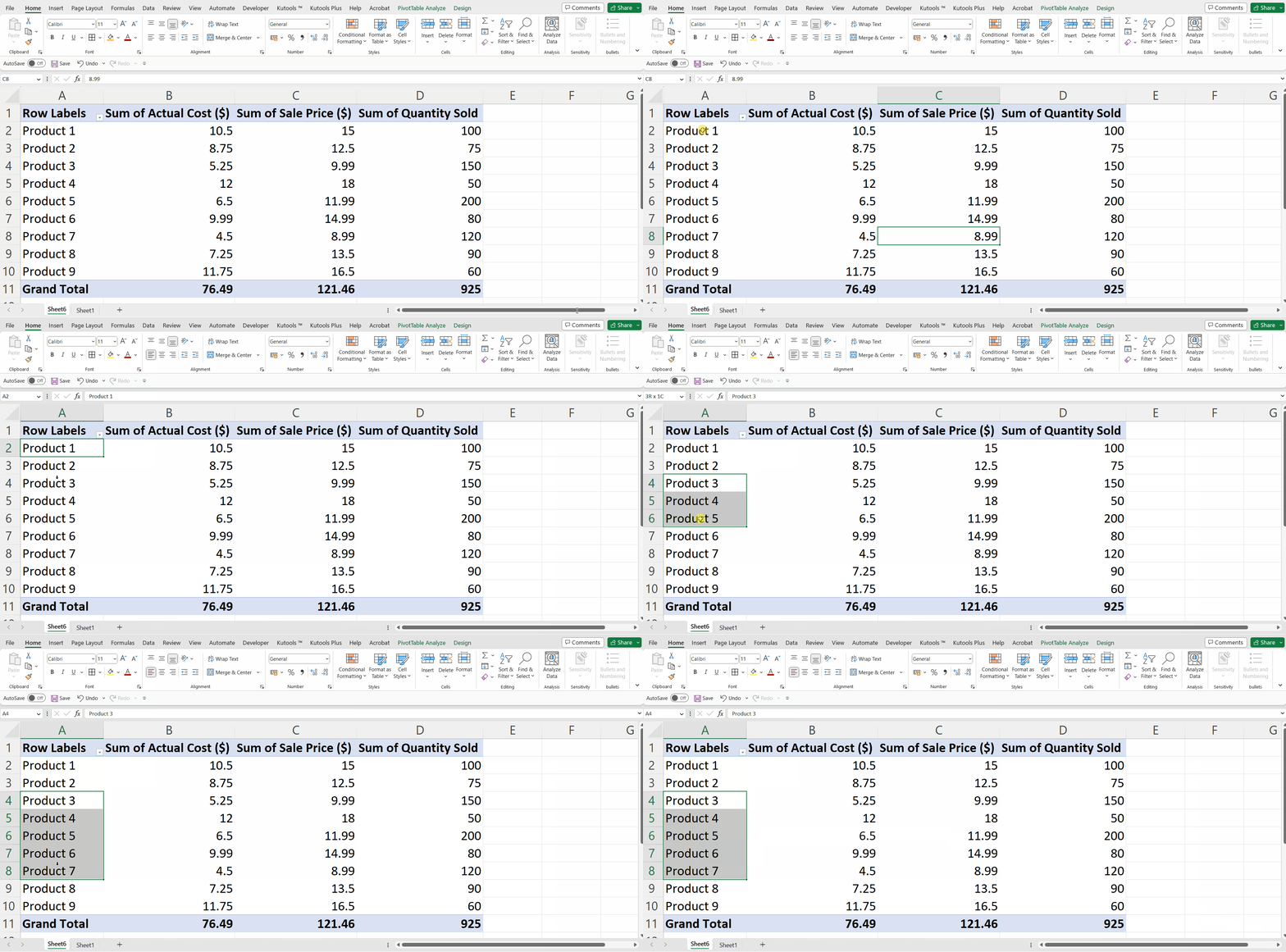
- Select the Items in the pivot table to be grouped.
Step 2 – Press ALT+SHIFT+ “➡”
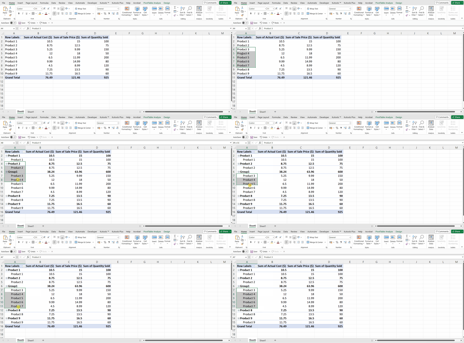
- Press ALT+SHIFT+ RIGHT ARROW (➡) keys.
- The selected items would be grouped.
Shortcut 4: Ungroup Items in a Pivot Table
We can also utilize the shortcut keys to ungroup the items when needed, this can be done by adopting the steps listed below.
Step 1 – Select the Items
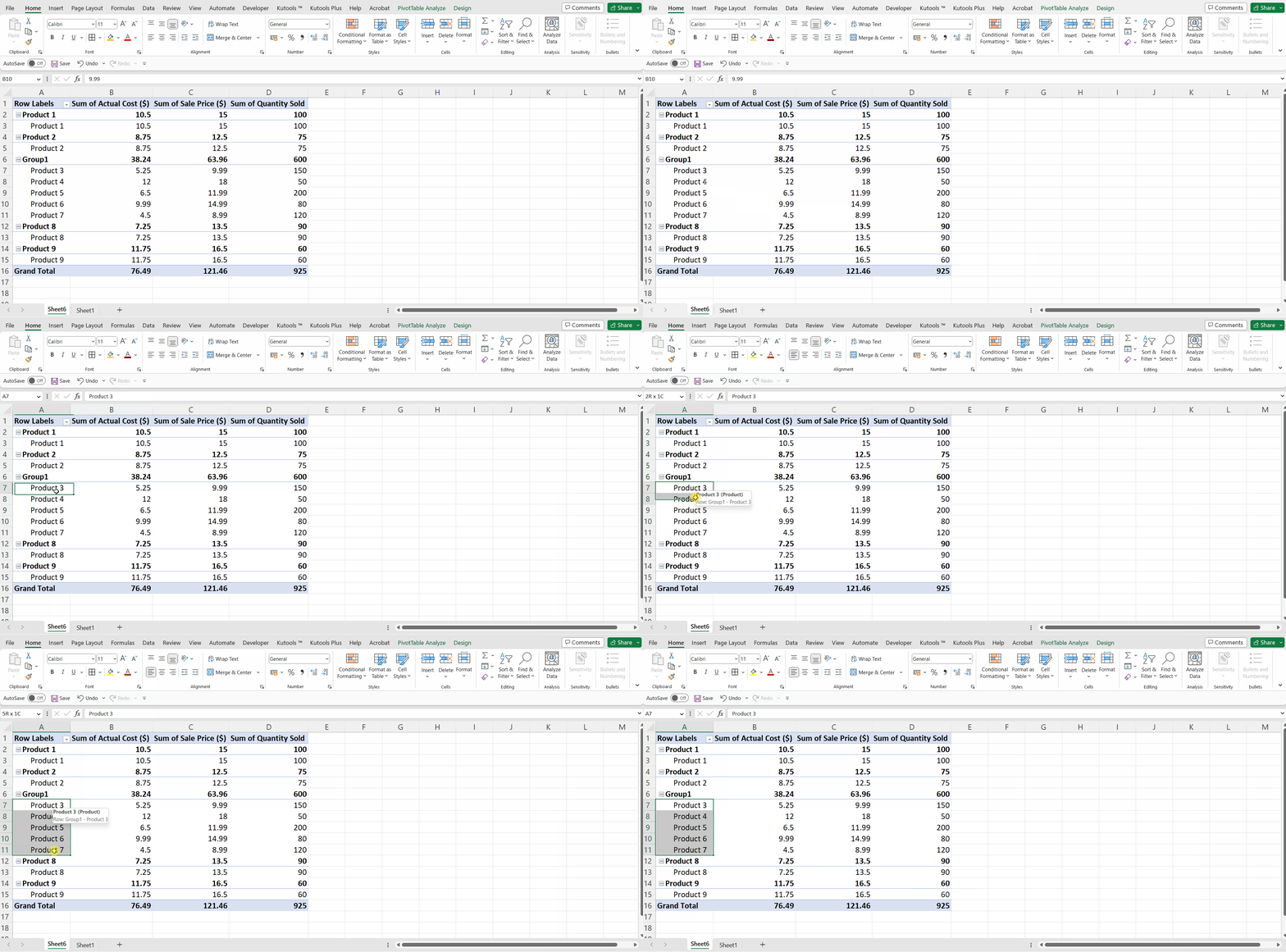
- Select the Items in the pivot table to be ungrouped.
Step 2 – Press ALT+SHIFT+ “⬅”
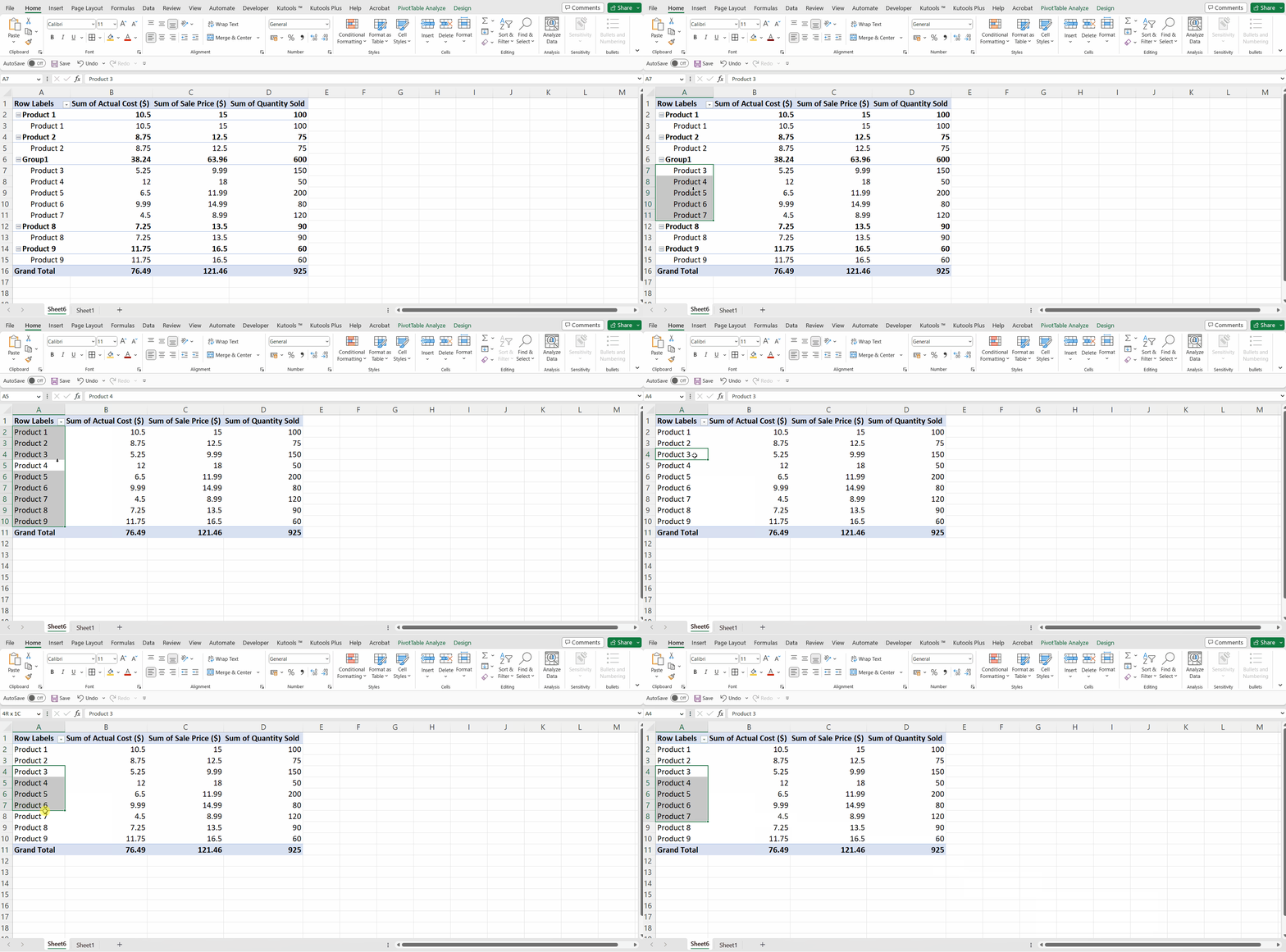
- Press the ALT+SHIFT+ LEFT ARROW (⬅) keys.
- The selected items would be ungrouped.
Shortcut 5: Hiding Items in a Pivot Table
Using shortcuts to hide items in a pivot table in Excel provides a quick and efficient way to selectively display or conceal specific data elements, enhancing data visibility and analysis.
Step 1 – Select the Items

- Select the items in the pivot table, you aim to hide.
Step 2 – Press CTRL+ “–”
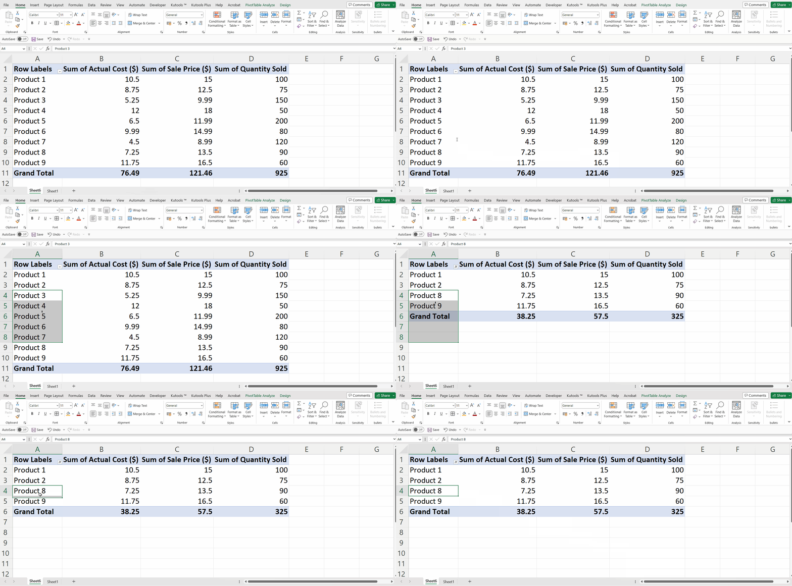
- Press the CTRL+ “–” keys on the keyboard.
- The selected items would be hidden.
Shortcut 6: Insert a Calculated Feild
A calculated field in a pivot table in Excel is a custom field that you can create by applying formulas to existing fields within the pivot table. Following is, how we can insert a new calculated field in a pivot table.
Step 1 – Click Anywhere on the Pivot Table
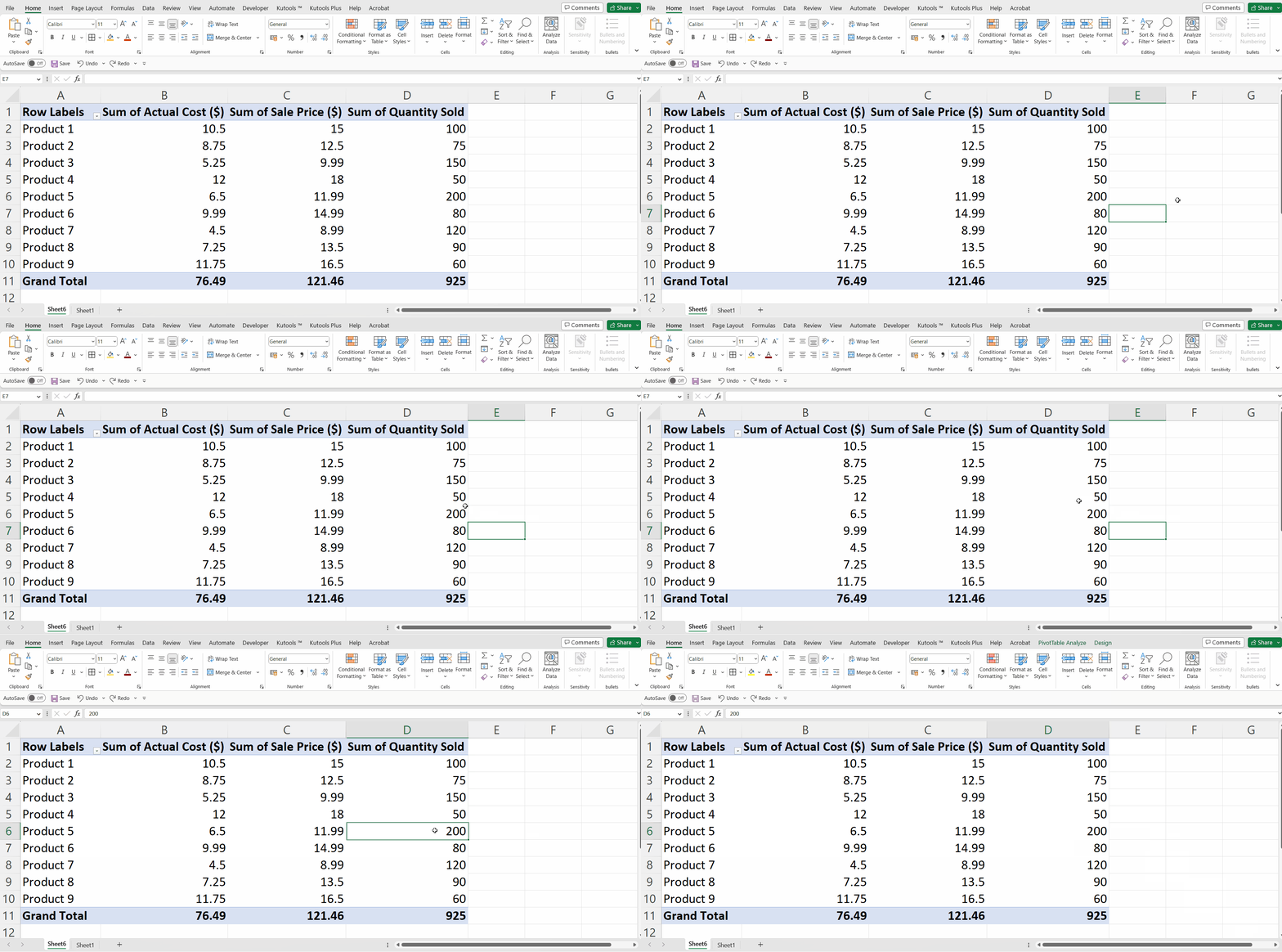
- Click anywhere on the pivot table.
Step 2 – Press the CTRL+SHIFT+ “=” Keys
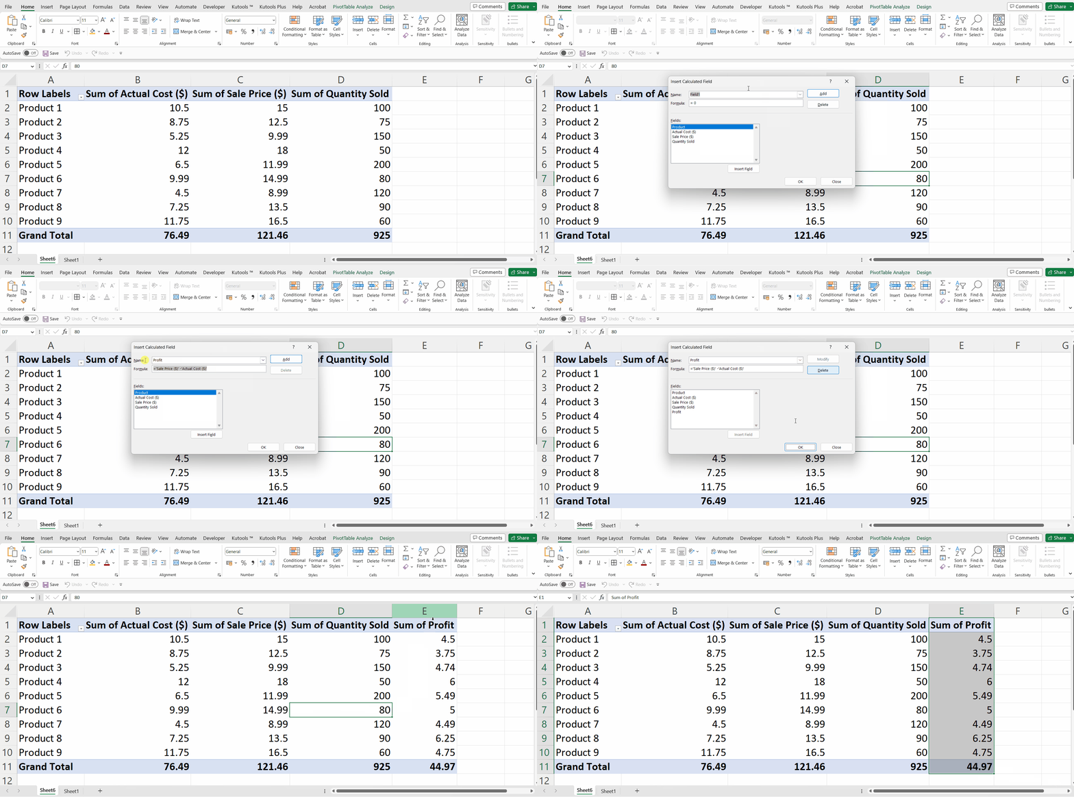
- Press the CTRL+SHIFT+ “=” keys on the keyboard.
- Insert the formula and create a calculated field.


