
How to use VLOOKUP with formatting
 By
SpreadCheaters
By
SpreadCheaters
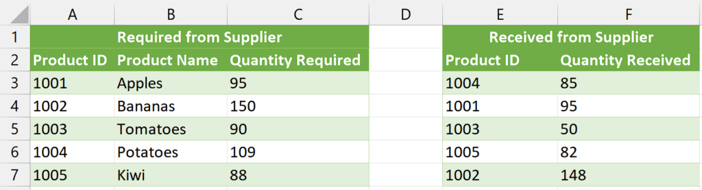
In this tutorial, we will explore how to utilize the VLOOKUP function within Conditional Formatting to format cells that indicate a discrepancy between the required quantities of products and the quantities received. The dataset includes Product IDs, Product names, the required quantities, and the quantities received. By applying this technique, we can easily identify instances where the supplied quantities fall short of the required amounts provided by the supplier.
Combining VLOOKUP with conditional formatting expands the capabilities of both features, allowing you to analyze, validate, and visualize data more effectively. It provides a dynamic and interactive way to format cells based on the results of the VLOOKUP function, enhancing data interpretation and decision-making.
Step 1 – Select the Range
– Select the range of cells on which you wish to apply the conditional formatting.
– For example, we have selected the range C3:C7.
Step 2 – Add a new Rule
– Navigate to the “Home” Tab and click on the “Conditional Formatting” Command button in the “Styles” group.
– It will open a drop-down list containing several options.
– Now, click on “New Rule” to open the “New Formatting Rule” dialogue box.
– From the Dialogue box, select the “Use Formula to determine which cells to format” option.
Step 3 – Write the formula
– Now, we will write the following formula in the dialogue box,
=VLOOKUP(A3,E3:F7,2,FALSE)<C3
Here is the breakdown of the formula:
VLOOKUP: It is a built-in function in Excel used to search for a value in the leftmost column of a table and retrieve a corresponding value from a specified column in the same row.
A3: It represents the lookup value. In this case, it is the value being searched for in the leftmost column of the table.
E3:F7: This is the range of cells that defines the table from which the VLOOKUP function will search for the lookup value. The leftmost column of this range should contain the values to be searched.
2: It specifies the column number in the table from which the function should retrieve the corresponding value. In this case, it will retrieve the value from the second column of the specified range (E3:F7).
FALSE: It is the last parameter of the VLOOKUP function, known as the “range_lookup” or “exact match” parameter. By setting it to FALSE, we are instructing the function to perform an exact match and return the corresponding value only if an exact match is found.
<C3: This is a comparison operator that checks if the value returned by the VLOOKUP function (the quantity received) is less than the value in cell C3 (the required quantity).
Step 4 – Format the cells
– After writing the formula, click on the “Format” option.
– You can select any format for the cells that meet the condition.
– For instance, we have selected the cells to be formatted as Bold with Red Fill and light grey Font color.
– Then, click on “OK” and your formatting will be applied.


