How to compare one column to another in Excel

Comparing one column to another in Excel involves checking if the values in one column are the same or different from the values in another column. This can be done using a variety of comparison operators or functions. comparing columns in Excel is an important data analysis and management tool that can help you validate data, identify duplicates, troubleshoot errors, and gain insights from your data.

Our dataset includes a list of car names that are present in two separate garages, each garage being represented by a different column. We want to compare the two garages using various conditions based on the car names. To do this, we have four different methods available to us that are explained below:

Method 1: Compare Columns using Equals to Formula

Step 1 – Select the Cell

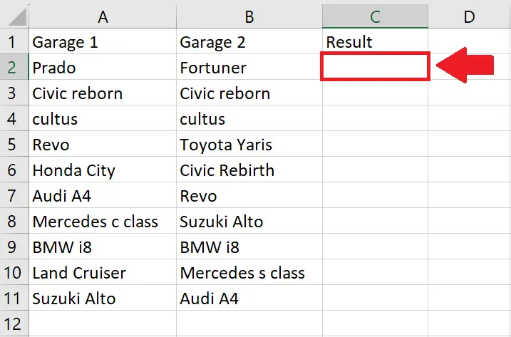
• Click on the cell where you want to show the result

Step 2 – Type the Formula 

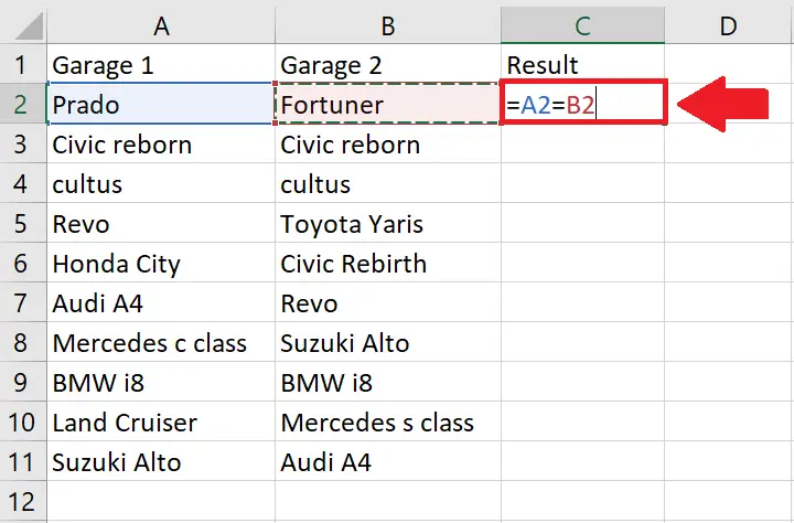
• Type Equal to sign (=) in the selected cell
• Then type the following formula:
• =A2=B2

Step 3 – Press the Enter key

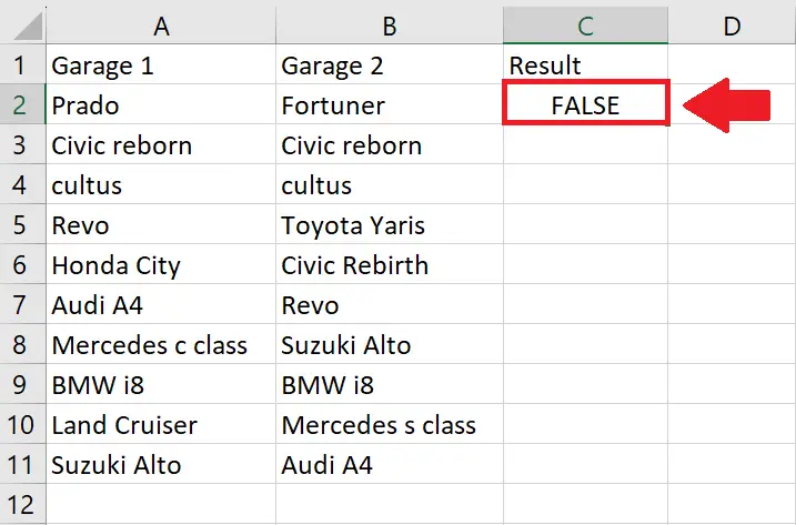
• After typing the formula, press the Enter key to get the required result

Step 4 – Apply the Formula to complete the column

• After pressing the Enter key, drag the cell to the last cell of the column to apply on the complete column

Method 2: Compare Columns using the Duplicate Conditional Fomating option

Step 1 – Select the Columns

• Select the complete columns that you want to compare

Step 2 – Click on the Conditional Formatting option

• After selecting the columns, click on the Conditional Formatting in the Styles group of the Home tab and a dropdown menu will appear

Step 3 – Click on the Highlight Cell Rules option

• From the drop-down menu, click on the Highlight Cell Rules option and a right-side menu will appear

Step 4 – Click on the Duplicate Option

• From the right side menu, click on the Duplicate Option and a dialog box will appear

Step 5 – Select the Color

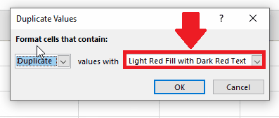
• Select the Color from the box next to the Values with the option
• Here we have selected red color you may select any other color you want

Step 6 – Click on OK

• After selecting the color, click on OK to get the required result

Method 3: Compare Columns using the Unique Conditional Fomating option

Step 1 – Select the Columns

• Select the complete columns that you want to compare

Step 2 – Click on the Conditional Formatting option

• After selecting the columns, click on the Conditional Formatting in the Styles group of the Home tab and a dropdown menu will appear

Step 3 – Click on the Highlight Cell Rules option

• From the drop-down menu, click on the Highlight Cell Rules option and a right-side menu will appear

Step 4 – Click on the Duplicate Option

• From the right side menu, click on the Duplicate Option and a dialog box will appear

Step 5 – Select the Unique option

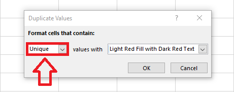
• In the box below the Format Cell that Contain option, select the Unique option

Step 6 – Select the Color

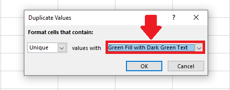
• After selecting the Unique option, select the color in the box next to the Values Wirth option
• Here we have selected green color, you may select any other color you want

Step 7 – Click on OK

• After selecting the color, click on OK to get the required result

Method 4: Compare Columns using the IFERROR function with the Vlookup function

Step 1 – Select the Cell

• Click on the cell where you want to show the result

Step 2 – Type the Combination of Functions

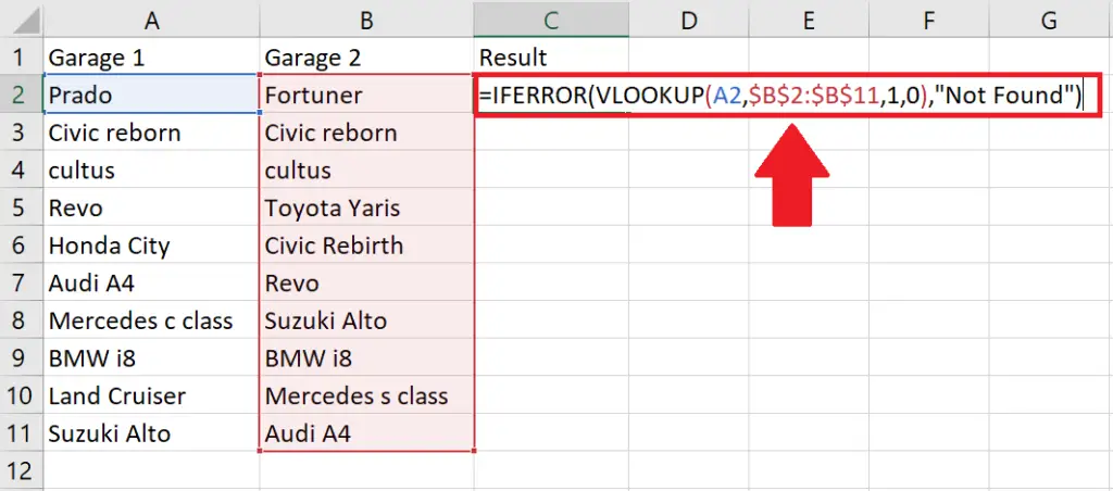
• After selecting the cell, type the following combination of functions:
• =IFERROR(VLOOKUP(A2,$B$2:$B$11,1,0),”Not Found”)

A2 is the cell containing the value being looked up

$B$2:$B$11 is the range of cells where the lookup value will be searched for

1 specifies that the function should return the value from the first column of the lookup range

0 means that the lookup should be exact

“Not Found” is the custom error message that will be returned if the lookup value is not found.

Overall, the formula is looking up the value in cell A2 in the range B2:B11, and if it finds a match, it returns the value. If it doesn’t find a match, it returns the custom error message “Not Found”.

Step 3 – Press the Enter key

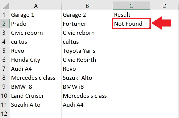
• After typing the Function, press the Enter key to get the result

Step 4 – Apply on the complete Column

• After getting the result in the cell, drag it to the last cell of the column to apply the same functions to complete the column