
How to use SUMIF not blank in Excel
 By
SpreadCheaters
By
SpreadCheaters
The importance of the SUMIF not blank functionality in Excel lies in its ability to perform calculations while excluding blank or empty cells. using the SUMIF not blank functionality, you can perform more accurate calculations, gain insights from your data, and create reliable reports in Excel.
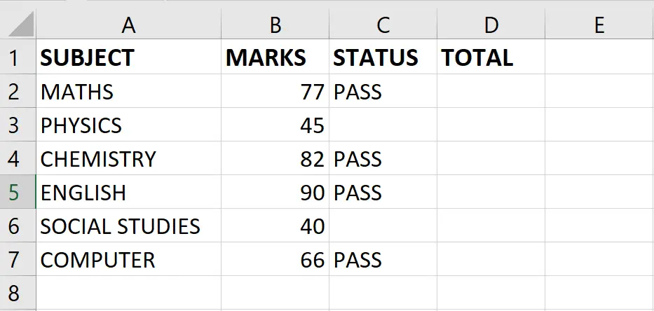
In our dataset, we have student results with subject names, marks, and a status column indicating whether they passed or failed. Passed subjects are labeled as “pass” in the status column, while failed subjects have blank cells. Our goal is to calculate the sum of marks for only the passed subjects, excluding the blank cells in the status column. We can achieve this using two methods: the SUMIFS function and the SUMIF function.
The SUMIF function in Excel is a powerful tool for calculating the sum of values based on specified criteria. It allows you to add up values in a range that meet a particular condition or criteria.
The general syntax of the SUMIF function is as follows:
=SUMIF(range, criteria, [sum_range])
- range: This is the range of cells that you want to evaluate against the criteria.
- criteria: This is the condition that determines which cells to include in the sum. It can be expressed as a number, text, logical expression, or cell reference.
- sum_range (optional): This is the range of cells containing the values you want to sum. If omitted, the range is used for summation.
Method 1: Sum if not blank use the SUMIF function
Step 1 – Select the cell

- Click on the cell where you want to show the result
Step 2 – Use the SUMIF function
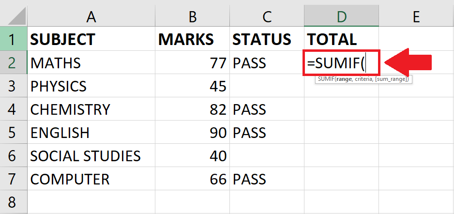
- After selecting the cell, use the SUMIF function by typing:
- =SUMIF(
Step 3 – Type the Arguments
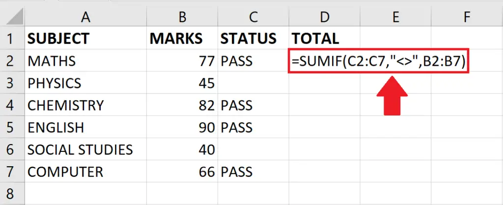
- Type the arguments of the SUMIFS function as follows:
=SUMIF(C2:C7,”<>”,B2:B7)
C2:C7: This is the range of cells you want to evaluate (in this case, cells C2 to C7).
“<>”: This is the criteria. The “<>” condition means “not equal to an empty string”. It includes only the cells in the range C2:C7 that are not blank.
B2:B7: This is the range of cells from which you want to sum the values. It corresponds to the values in B2 to B7.
Step 4 – Press the ENTER key
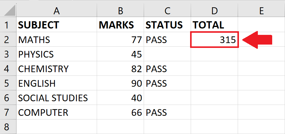
- After typing the arguments, press the ENTER key to get the required result
The SUMIFS function in Excel is an advanced version of the SUMIF function. It allows you to calculate the sum of values that meet multiple criteria simultaneously. With SUMIFS, you can specify multiple ranges and corresponding criteria to determine which cells to include in the sum.
The general syntax of the SUMIFS function is as follows:
=SUMIFS(sum_range, criteria_range1, criteria1, [criteria_range2, criteria2], …)
- sum_range: This is the range of cells containing the values you want to sum.
- criteria_range1: This is the first range of cells that you want to evaluate against the first criterion.
- criteria1: This is the first criterion or condition that determines which cells to include in the sum for criteria_range1.
- [criteria_range2, criteria2]: These are optional additional ranges and criteria to further refine the selection of cells for summation.
Method 2: Sum if not blank using the SUMIFS function
Step 1 – Select the cell
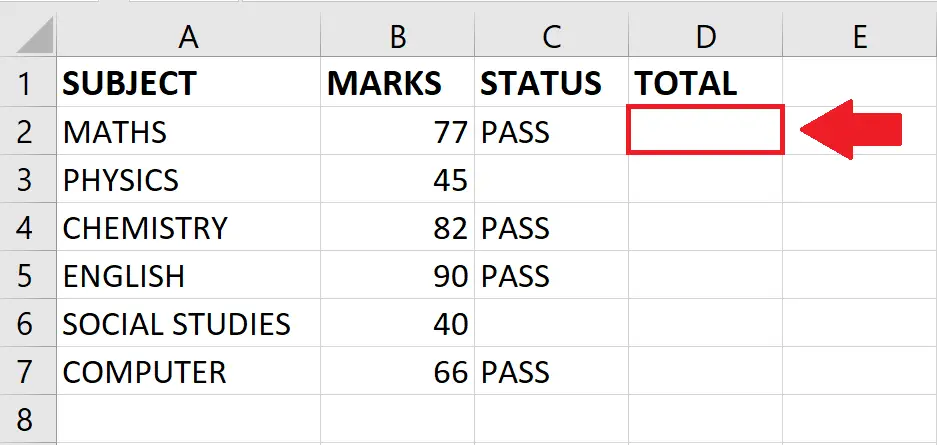
- Click on the cell where you want to show the result
Step 2 – Use the SUMIFS function
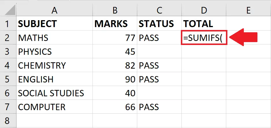
- After selecting the cell, use the SUMIFS function by typing:
- =SUMIFS(
Step 3 – Type the Arguments
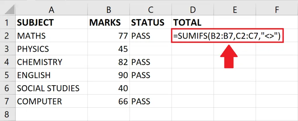
- Type the arguments of the SUMIFS function as follows:
- =SUMIFS(B2:B7,C2:C7,”<>”)
Step 4 – Press the ENTER key
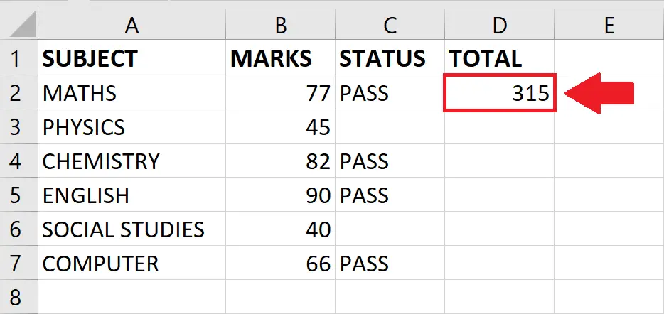
- After typing the arguments, press the ENTER key to get the required result


