
How to use SUMIF less than in Excel
 By
SpreadCheaters
By
SpreadCheaters
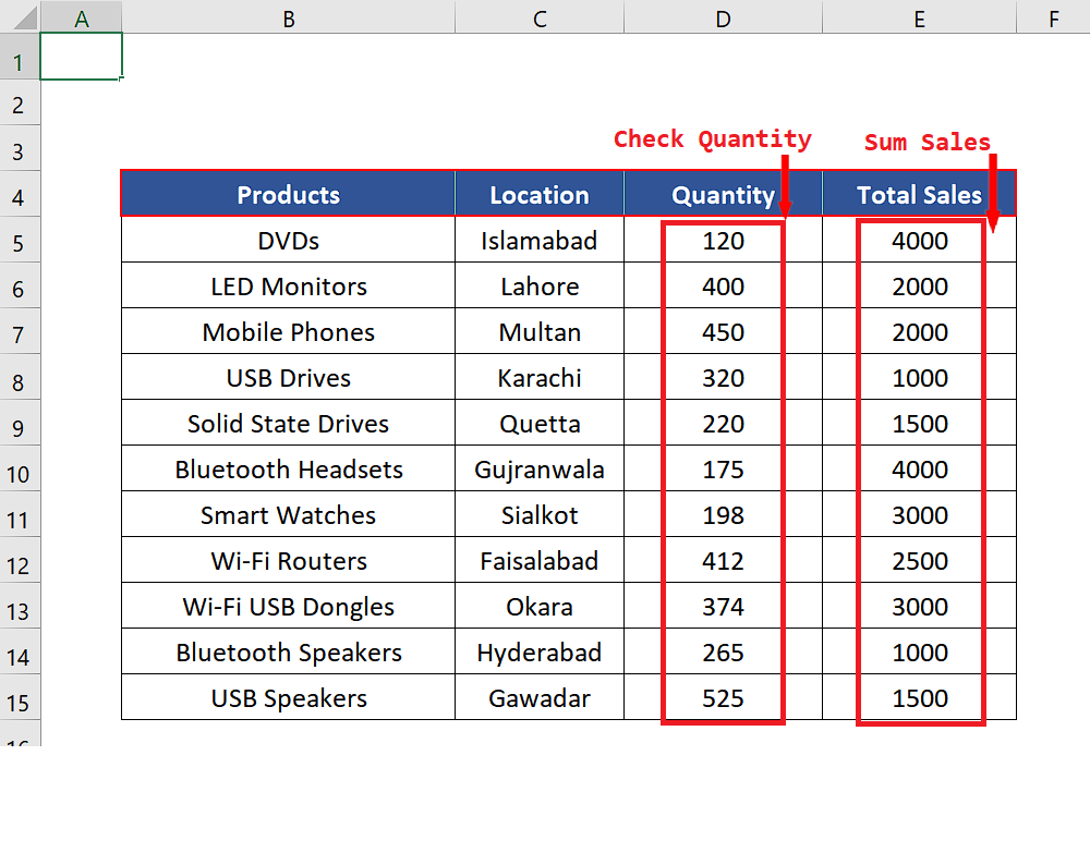
In today’s tutorial we’ll learn how to use the SUMIF function in Excel to sum all those values which are lesser than a specific value. Let’s look at the dataset given below. It contains the sales data of various products from various locations. We’ll sum the sales of all those items whose sold quantity is less than a particular value from the dataset shown above.
Follow along the steps mentioned below to learn how to use SUMIF with greater than condition in Excel. Let’s learn the syntax of SUMIF and see what parameters are required to use this formula properly.
Syntax of SUMIF
The syntax of the SUMIF formula is as follows,
=SUMIF(range, criteria, sum_range)
range:
This is the range which will be checked against the criteria. We’ll call it the criteria range. In our case this will be D5:D15.
criteria:
This is the condition that will be checked. The important thing to note here is that the criteria or condition will be written in text format i.e., inside double quotes. Even if it is a condition involving only numeric value comparison. Therefore, we can use “<450” or “<”&G5 to make the criteria value dynamically modifiable. In the latter case, G5 will hold the value which will be compared or checked inside the given range. The ampersand sign & concatenates the greater than symbol and the value from G5 and converts them in text format. Therefore, we can use this combination as the text condition inside the SUMIF function.
sum_range: This is the range (E5:E15 in our case) from which we’ll pick the values to add them whenever the condition inside the criteria range is met the corresponding value from the sum_range will be picked and added to the sum.

Excel is a very handy software tool for organizing and manipulating any type of datasets. It has many functions for calculations and data visualization. It also provides us with a lot of functions for logical decisions and then we can use the results of these functions to perform some mathematical calculations.
Step 1 – Choose a cell for dynamic criteria
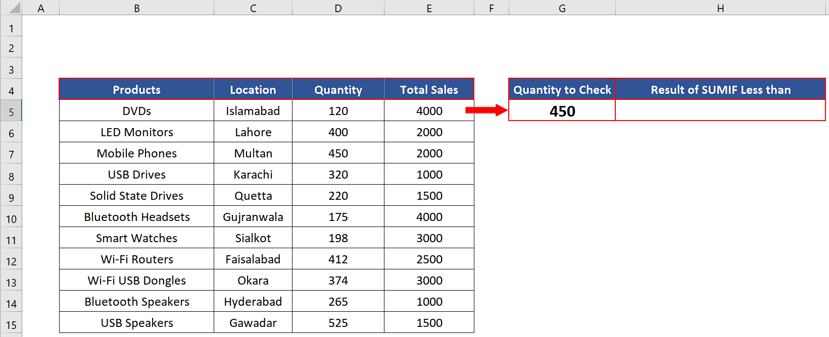
– Select a cell outside the data table.
– Give it a suitable name. For our example, we’ll use “Quantity to Check”.
– Choose an appropriate value which will be checked inside the criteria range. We’ll choose 450 as the checking criteria, as shown above.
Step 2 – Implement the formula with SUMIF
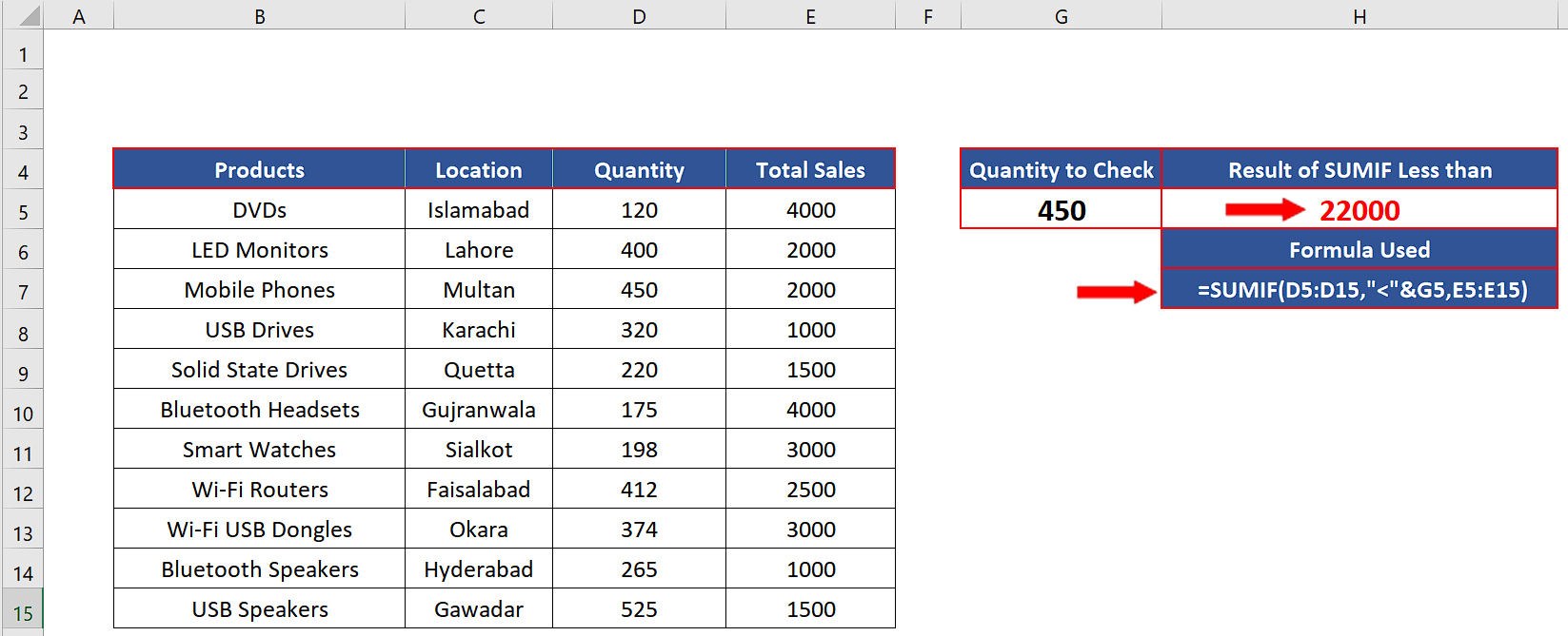
– We’ll use the following formula for checking and adding the sales values for all those items for which the sale quantities are less than 450, as shown above.
=SUMIF(D5:D15,”<“&G5,E5:E15)
Step 3 – Change the criteria dynamically
– We have set up the SUMIF function in such a way that when we change the value in cell G5, the SUMIF less than criteria will be updated and new results will be calculated automatically as shown above.


