
How to use SUMIF function with the condition “greater than 0”
 By
SpreadCheaters
By
SpreadCheaters
Suppose you have a dataset that contains information about the names of the medicines, the number of medicines that are sold, and the number of medicines that expired which aren’t sold. Now the values of sold medicines are positive and the values of expired medicines are negative values. The profit on sold products and loss on expired products is also mentioned.
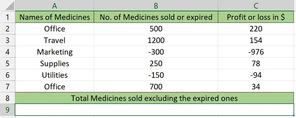
In this calculation, we will find the sum of the sold medicines excluding expired medicines. We’ll use the SUMIF function with the condition “greater than 0” to exclude any expired medicines (negative amounts).
- Understanding the formula
- The SUMIF function follows the syntax shown below:
=SUMIF(range, criteria, [sum_range])
The parameters of this function are as follows:
range: This is the range of cells that you want to evaluate.
criteria: This is the condition or criteria that determine which cells should be included in the sum. It can be in the form of a number, text, logical expression, or cell reference.sum_range (optional): This is the range of cells that you want to sum if the corresponding cells in the range meet the criteria. If you don’t provide a sum_range, the function will use the range parameter for summation.
The SUMIF function is a mathematical function commonly used in spreadsheet software, such as Microsoft Excel or Google Sheets, to calculate the sum of a range of cells based on specific criteria or conditions. It allows you to add up values in a range that meet a given condition.
Step 1 – Selection of cells

– Choose an empty cell where you intend to use the SUMIF function.
– This cell will be used to calculate the sum of values based on a specific condition of being greater than zero.
Step 2 – Writing the formula
– For writing the formula, type = in the cell you’ve selected.
– Then, type SUMIF and select the SUMIF Function by pressing the tab button on your keyboard.
– Then select the range of cells that will be tested to determine if they meet the criteria. This range will be taken as the first parameter range. For example, C2:C7 in this case.
– Then type a comma (,) and you will move to the second parameter criteria.
– In this parameter, type “>0” (quotes included) which basically tells us that this is the condition that would be applied to the first range, and on the basis of this requirement the second range’s values would be summed.
– Then type a comma (,) and you will move to the third parameter sum_range.
– After doing that, enter the range (for example, B2:B7) of which the values would be summed if it meets the condition applied to the range of the first parameter.
– Now that you have followed all the steps above, your formula would look like this, =SUMIF(C2:C7,”>0″, B2:B7)
Step 3 – Implementation of the formula
– Once you’ve done this, close the parenthesis and press Enter button.
– Now, the cells that met the condition of being greater than zero in column B would be summed as they will appear as a result and all the negative values would be excluded.
– As you can see that the medicines sold are summed only which were in positive values and all the expired medicines which were present in negative values weren’t summed which satisfies the condition of the answer being greater than 0.


