How to unlink Excel sheets 

While working in Excel and handling a large amount of data, we often need to create links in our sheets to redirect users to other sheets. To link sheets in a workbook, we use the hyperlink function. Unlinking sheets allow you to separate specific data or information from the rest of the workbook. This can be useful when you want to share or analyze detailed data independently without affecting or being affected by other sheets in the workbook. Unlinking sheets can help protect sensitive or confidential data. 

We can unlink sheets in Excel in two ways. One way is to remove hyperlinks that connect two sheets. The other way is to break the links that connect the data between two sheets. In this tutorial, two simple methods to break links between two sheets are discussed: 

Method 1 – Copying and pasting  as values only 

One method to break links between Excel spreadsheets is to remove the formulas that connect the sheets and paste the values only. Doing so will break the links between spreadsheets and the data will no more be linked with each other. Consider the following dataset that contains the details of the final examination results of four students of a class. In the following dataset, we need to calculate the percentage also and for calculating the percentages, we need values of total marks and obtained marks, that are present in other spreadsheets. In this particular workbook, four more sheets are also present that contain mark sheets of the students. You can see in the formula bar that the cell has been taken from sheet “SA”, named with the initials Sophia Anderson. When we include cells from other sheets, the sheets automatically become linked. 

Step 1 – Identify Formulas used in the sheet 

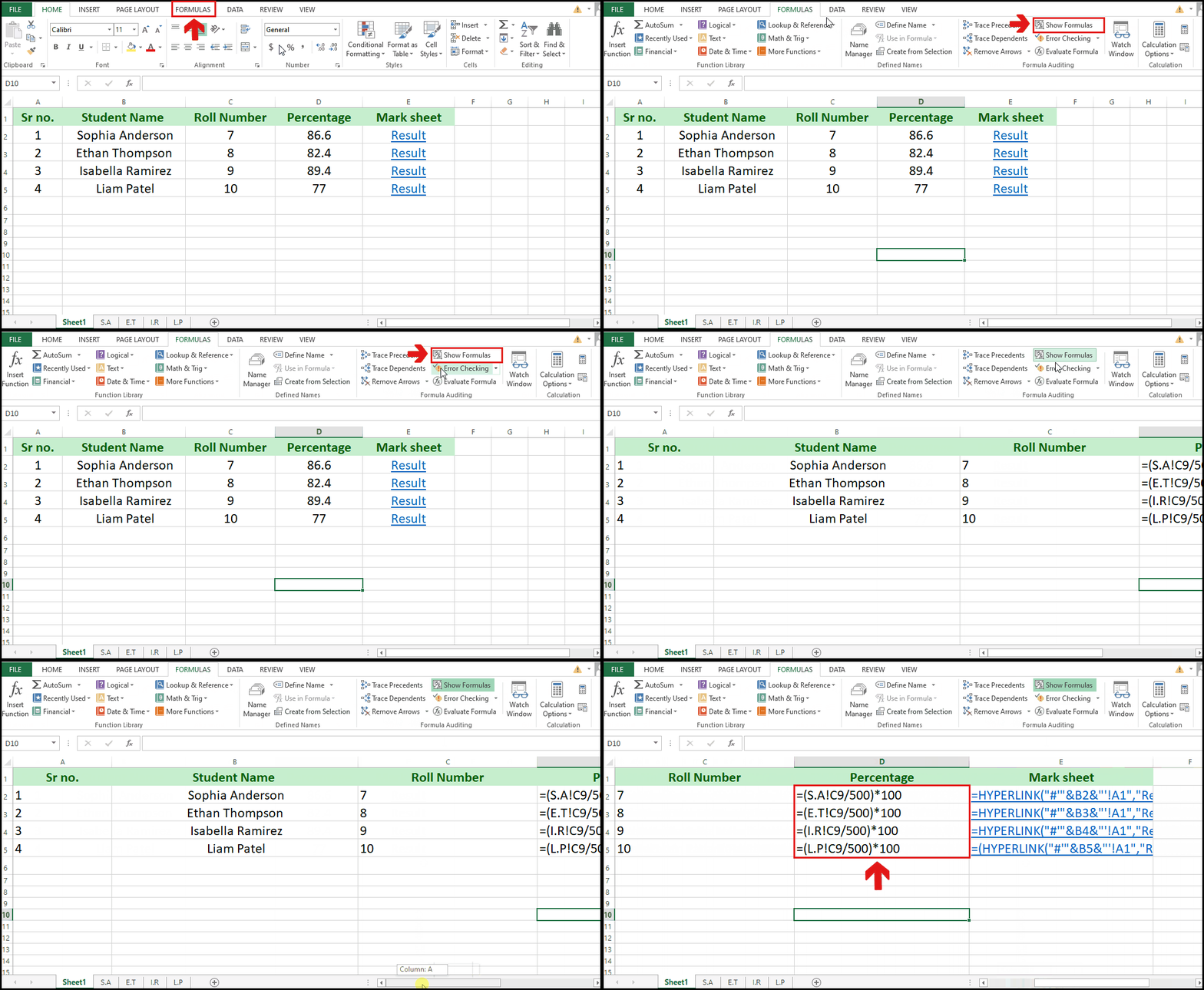
• If you know the cells in which the formulas are used that link the sheets, then you don’t need to follow this step. 
• However, if you get a random dataset and are asked to break links between them, then you need to identify the cells with formulas first. 
• Therefore, select the sheet in which you want to check the formulas. 
• Go to the “Formulas” tab. 
• Locate the “Formula Auditing” group. 

• Click on the “Show Formulas” action button to see the used formulas. 
• You can see in the formula bar that the cells from another sheet are used in the formula. 

Step 2 – Select the cells or columns with formulas and copy them 

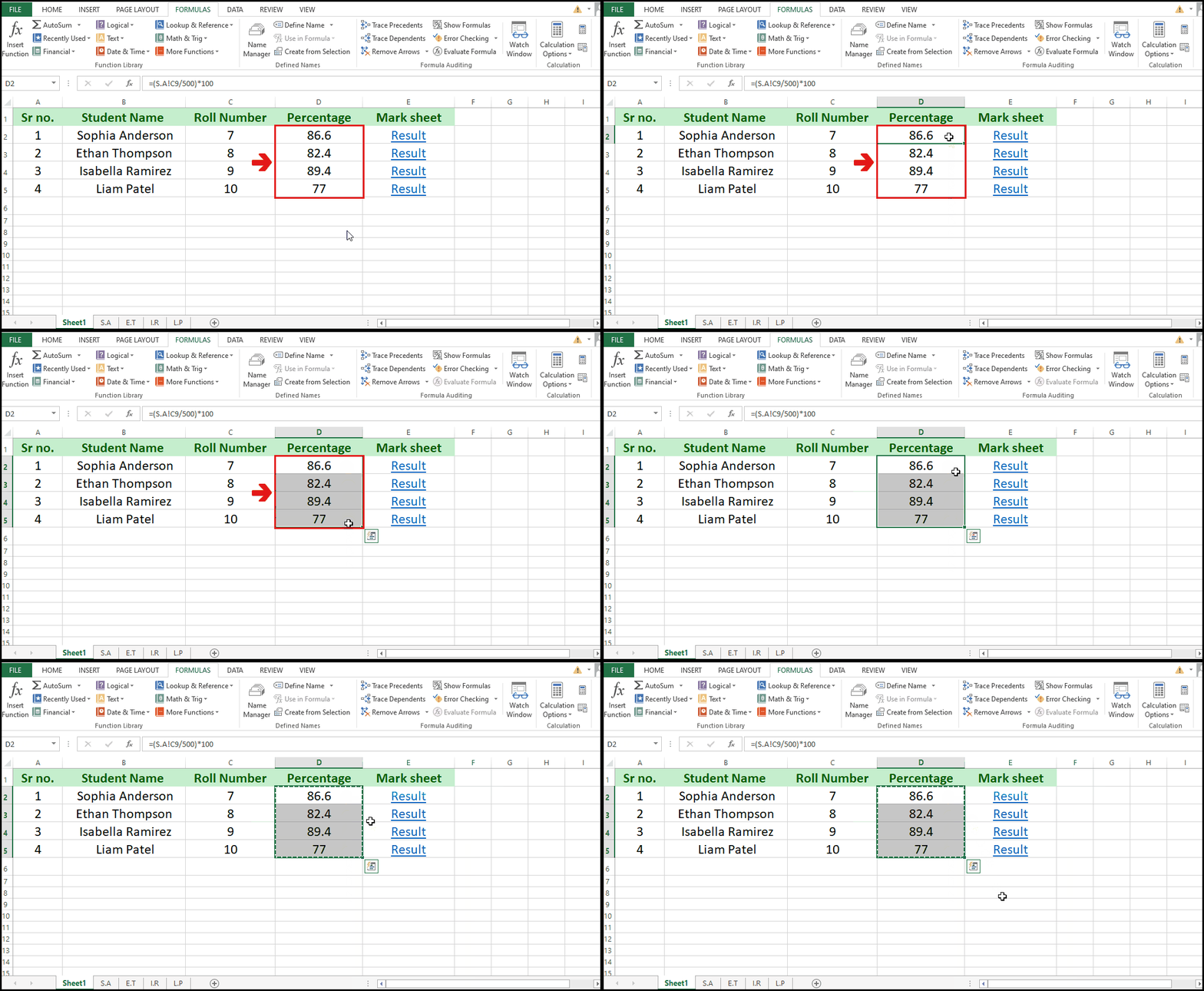
• After identifying the cells or column that has the formulas that link the two sheets, move your cursor to the cells or column. 
• Click and drag to select the cells or columns. 
• After selecting, right-click on the selected cell and click on “Copy”, or simply press Ctrl+C from the keyboard. 
• In this case, the range of cells that contain linking formulas is from D2 to D5. 

Step 3 – Paste it as “Values Only” 

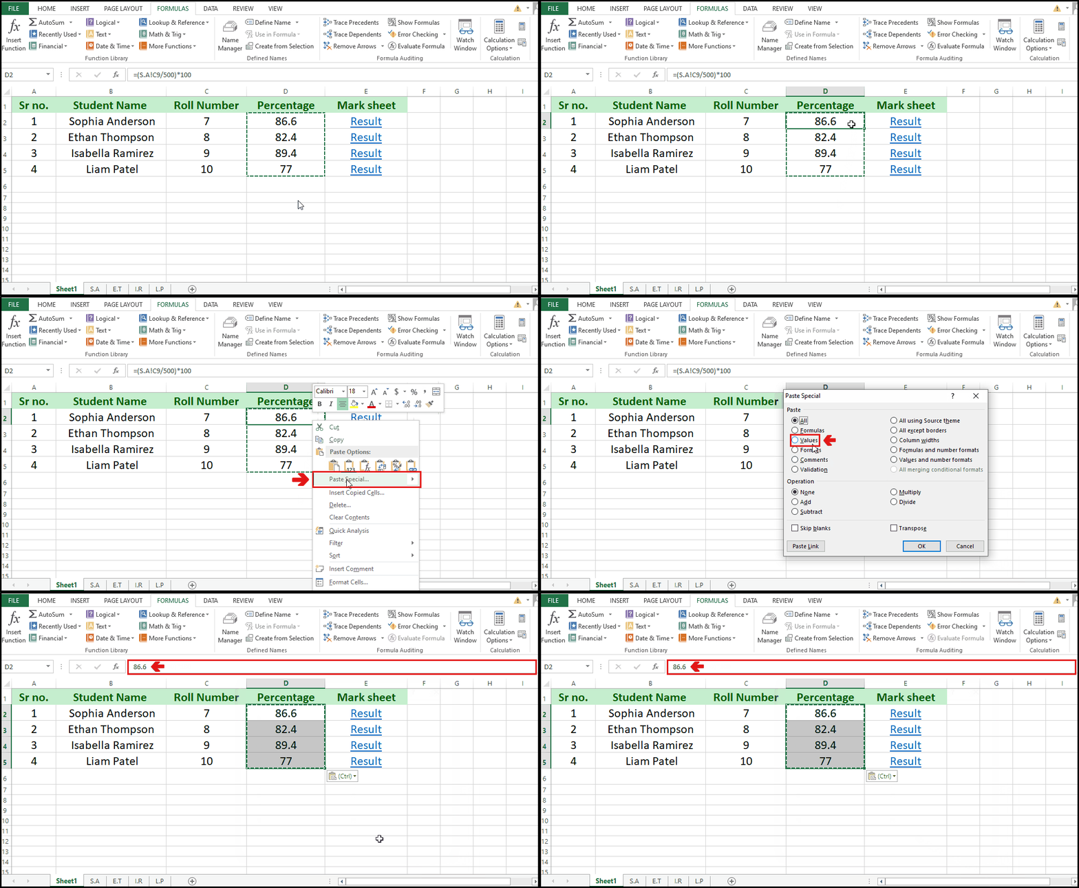
• Move your cursor to the first cell that you copied. 
• Right-Click on it. 
• Click on “Paste Special”. 
• Click on “Values”. 
• Click on OK. 

• You can see in the formula bar that the formula is replaced with values,  and the sheets have been unlinked. 
• Alternatively, you can use the shortcut keys CTRL+ALT+V+V and then press Ok. 

Method 2 – Removing the hyperlinks 

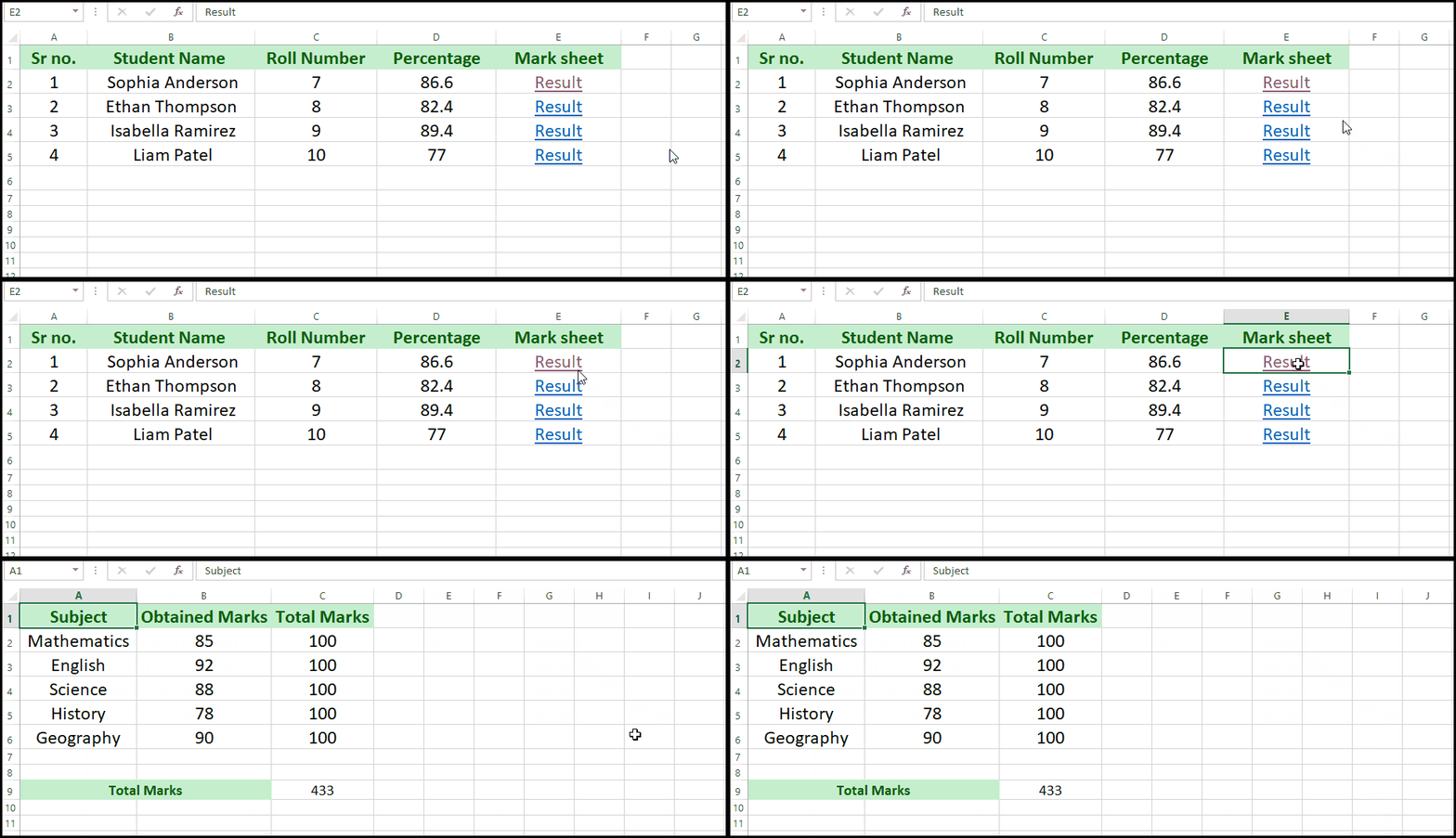
When we create hyperlinks in spreadsheets that connect one spreadsheet to another, a link is created between them. There are many ways to remove hyperlinks in Excel. But a very simple and easy way to remove hyperlinks is to change the style of the text. Consider the following dataset that contains the result of the final examination of four students. The hyperlinks to the mark sheets of students are given in a separate column.  

Step 1 – Select the cell that contains hyperlinks 

• Move your cursor to the cell that contains the hyperlink and select it. 
• In this case, the range of cell that contains hyperlink is from E2 to E5. 

Step 2 – Change the style of the text 

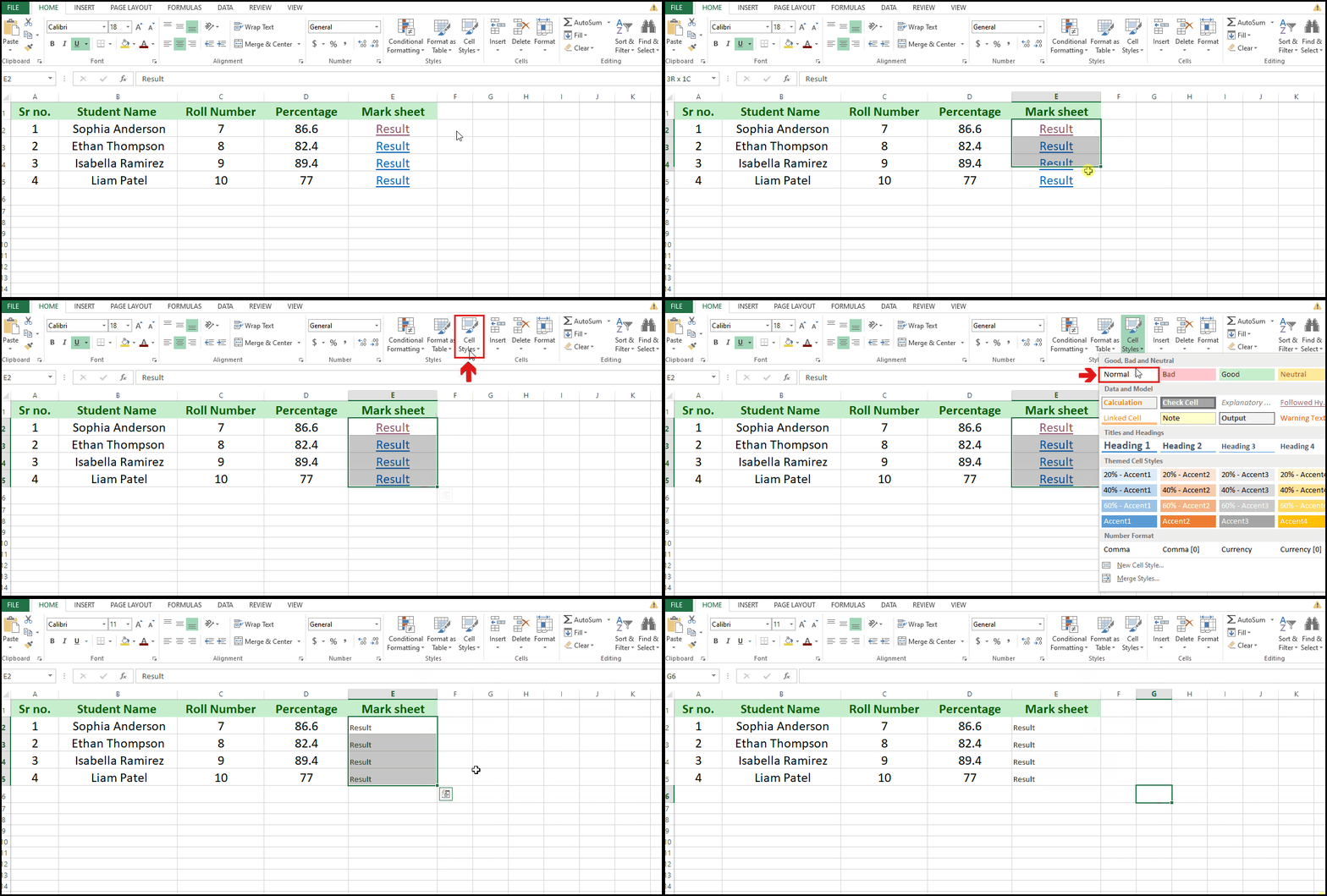
• After selecting the cells, Go to the “Styles” group of the “Home” tab. 
• Click the style from “Hyperlink” to “Normal”. 
• This will remove the hyperlinks from the selected cells and thus break the link between spreadsheets.