How to turn data into a table form in Excel.
Let’s use a data set that details a company’s sales for the purposes of this demonstration. The information is broken down into columns for “Product Name,” “Price,” “Quantity Sold,” and “Total Sales.” We can improve this data’s visual appeal and make use of table-specific features by turning it into a table.
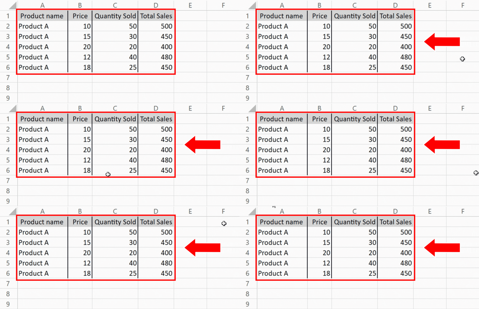
Data organization and analysis are made simple with the help of Excel, a powerful spreadsheet program. You can transform your data into a table format using Excel, which is a useful feature. Data filtering, sorting, and formatting are all made simple with tables in Excel. To enable you to utilize Excel’s table functionality to its fullest, we will guide you through the process of creating a table from your data in this documentation.
Step 1 – Select the data
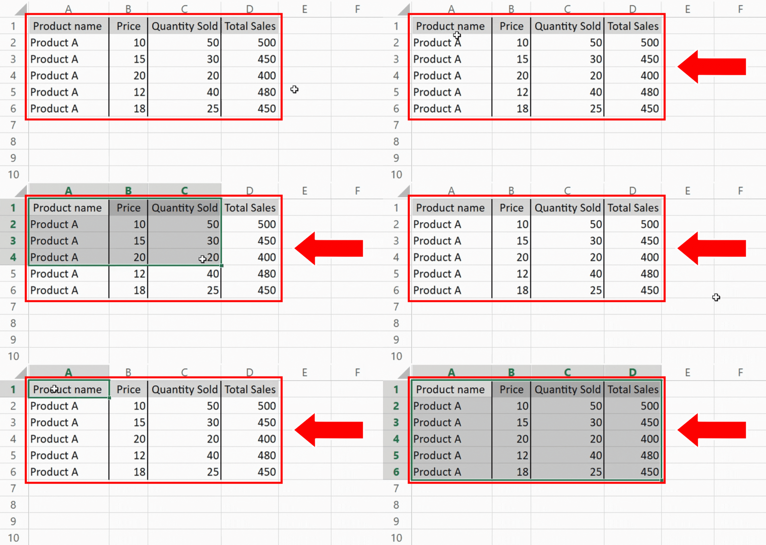
– Open the workbook containing the data you want to turn into a table in Excel after starting it, go to the worksheet where the data are located.
– The range of cells you want to include in the table should be determined. Make sure you choose all the necessary rows and columns.
– To create a selection box that includes all the desired cells, move the cursor to the last cell of the range while continuing to hold down the left mouse button, To complete the selection, release the mouse button.
Step 2 – Access the Table Creation Option
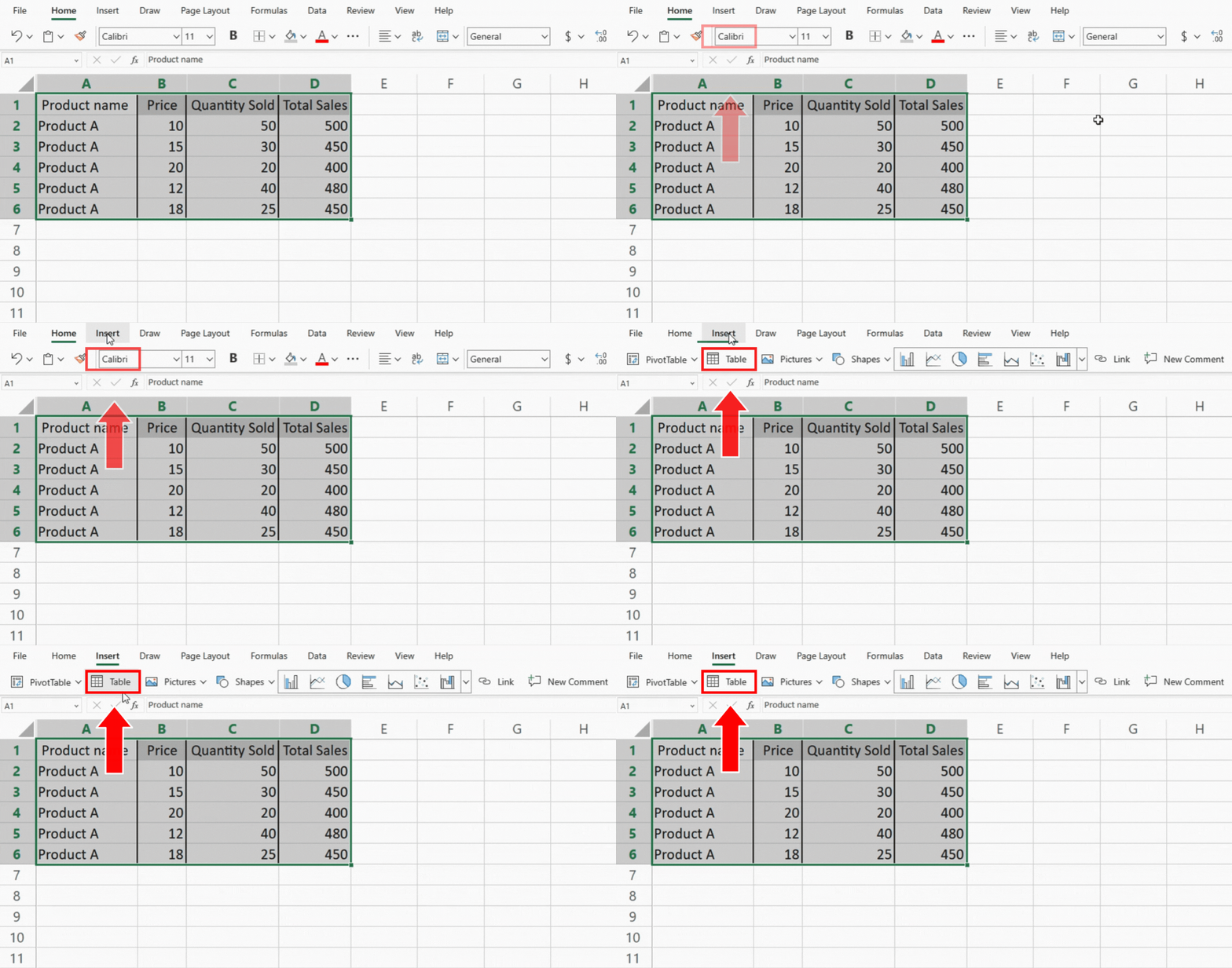
– Click on the Insert tab at the top of the Excel window after selecting the data range.
– In the ribbon, look for the “Tables” group. It is typically found on the “Insert” tab’s left side.
– The Table button is located in the Tables group. To continue, click it.
Step 3 – Create the Table
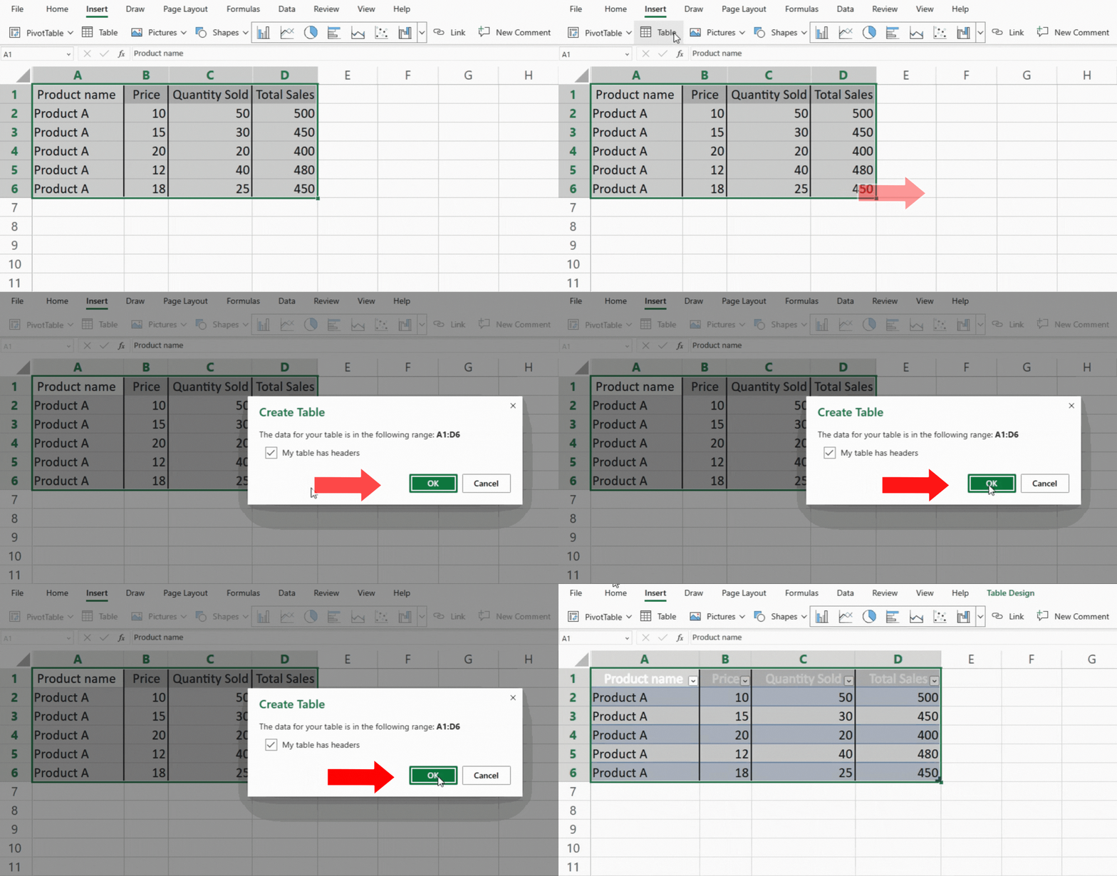
– Clicking the table button will open a dialog box.
– If your data set has column headers, check the “My table has headers” box. Excel will be able to handle the top row as the header row as a result.
– Verify if the selected range that is shown in the dialogue box accurately matches your data. If necessary, modify.
– To create the table, press the OK button.
Step 4 – Adjust Column Width
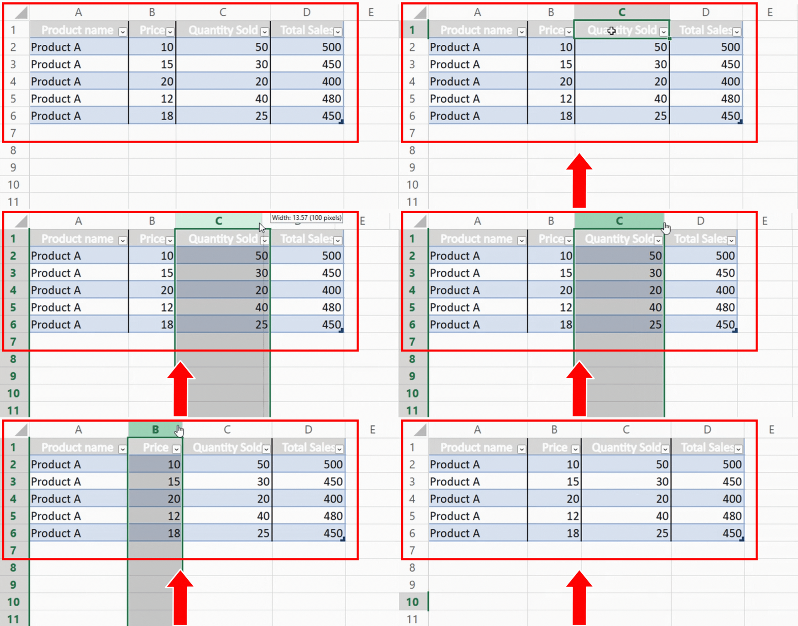
– Your table’s columns should be resized so that the header names are clearly visible.
– Drag the column borders to the desired width to accomplish this.
Step 5 – Customize Table Style

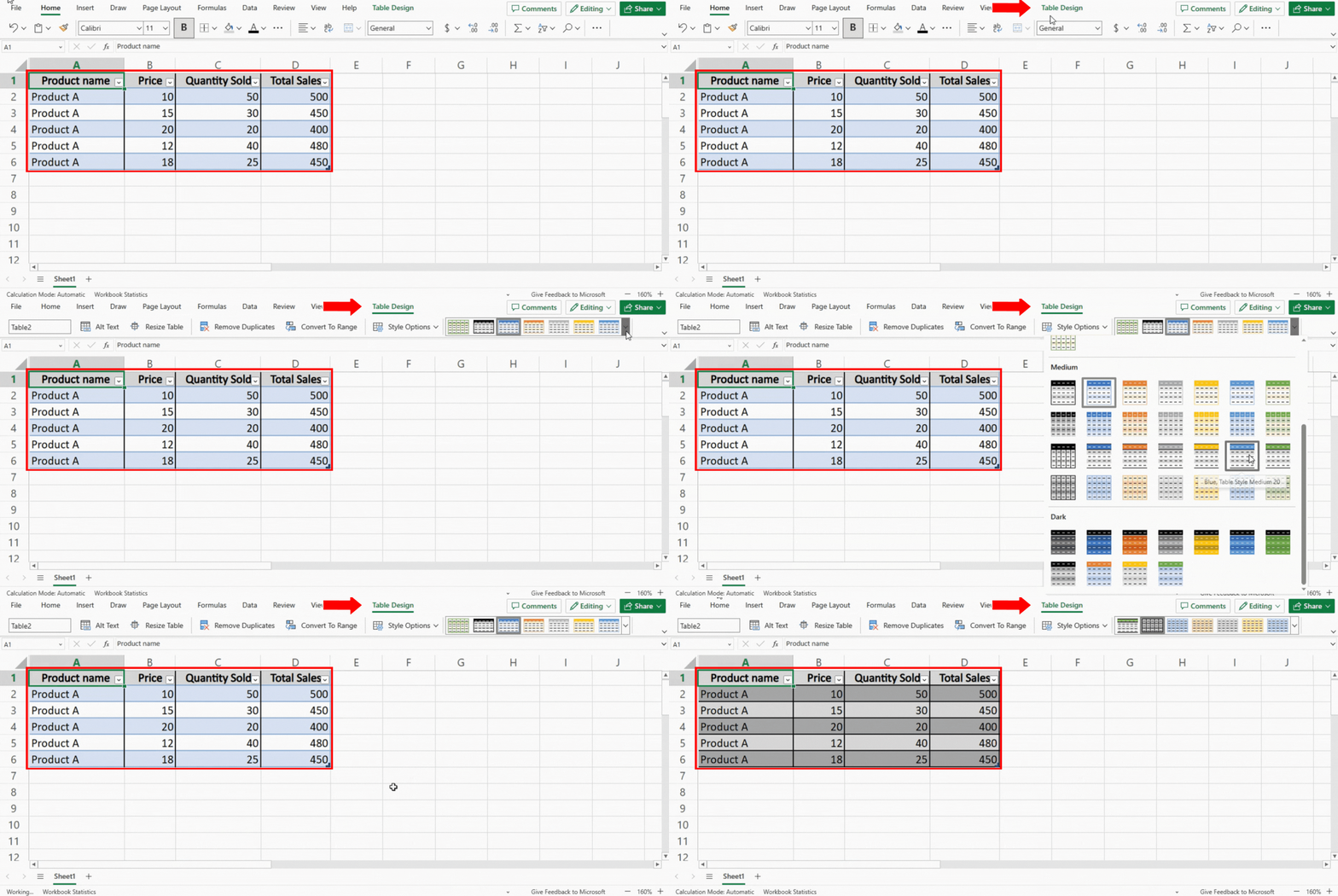
– To open the Table Tools tab in the Excel ribbon, click any cell in the table, and go to the Design tab under the Table Tools tab.
– Find the Table Styles group and peruse the various style/color options there.
– To see a preview of how each style will appear on your table, hover over it.
– To apply the chosen style to your table, click on it.


