
How to filter multiple columns in Excel
 By
SpreadCheaters
By
SpreadCheaters
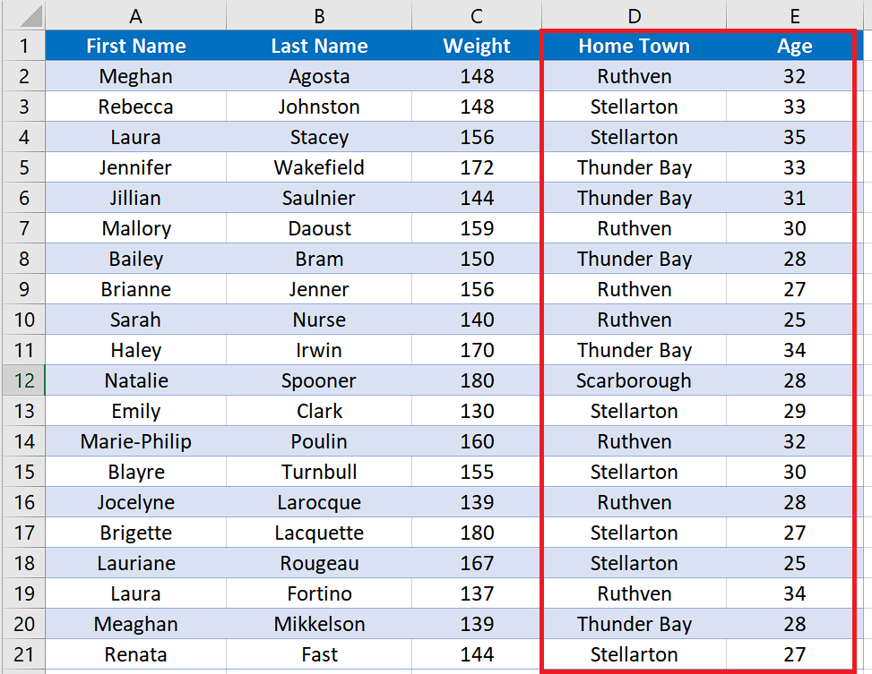

Excel comes with many functions to analyse data sets and it also provides tools and functions to sort and rearrange data for better representation. Application of filters is one such tool which rearranges big data sets to show only the desired data. The conventional filter available in Excel can only filter by one column at a time. In today’s tutorial, we’ll learn how to filter multiple columns simultaneously.
Step 1 – Create a second sheet and create filter criteria
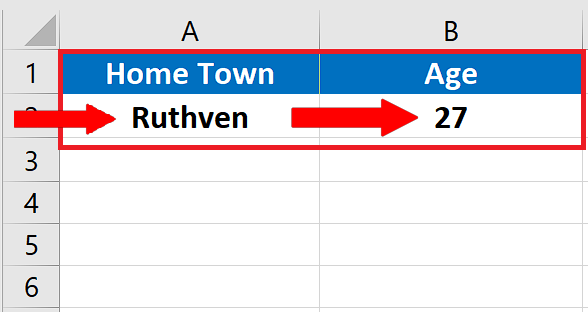
– First of all create a second sheet by pressing SHIFT + F11 keys. Rename the sheet to Filter Criteria and create the following criteria.
Step 2 – Create an advanced filter for multiple columns
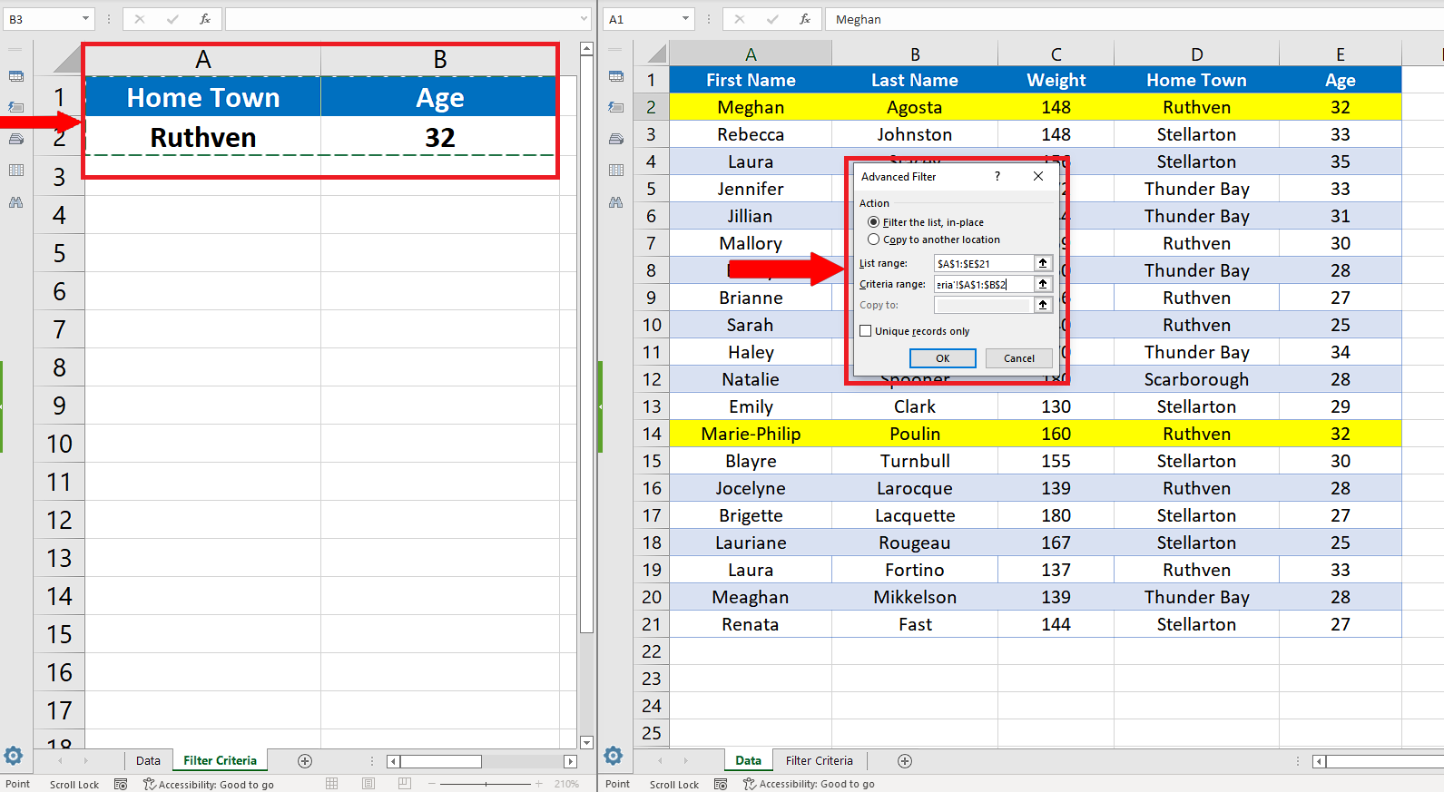
– The best and easiest way to filter multiple columns is to create an advanced filter and then add a criteria to filter multiple columns simultaneously.
– For this purpose, first select the data range on which you wish to apply the filter.
– Then go to the Data tab from the list of tabs at the top. Locate the Sort & Filter group and click on the Advanced option.
– This will bring up another dialog box named Advanced Filter, asking you to choose a criteria range.
Choose the cells on the Filter Criteria sheet as shown above.
Step 3 – Implement advanced filter for multiple columns to meet multiple conditions
– As soon as you click OK after choosing the right cells for the criteria you will have the data range filtered. The current filter implements an “AND” logic and as per the filter criteria, only those players were chosen whose HomeTown was “Ruthven” and whose Age was “32”. The rows containing this information were already marked with yellow colour so that we can check the output of our filter.
Step 4 – Implement filter with an OR condition for multiple columns
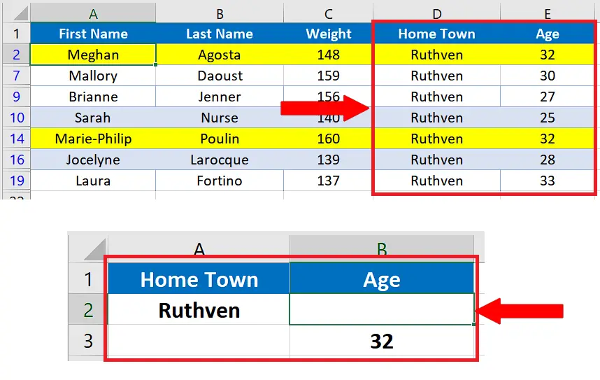
– We can play with our filter criteria a little bit and this time we’ll create a filter to choose the players who are either from Ruthven or have age 33.
– To do this simply move the number in the cell B2 to B3 in the Filter Criteria sheet.
– Repeat the process of creating the filter as described in the previous step and the data will be filtered as per the new criteria.
– We can see from the result of the filtered data that we got the players who are either from Ruthven or have age 32.
So this is how we can create an advanced filter which can filter multiple columns simultaneously.


