How to transpose data in Google Sheets.

Google Sheets is a powerful spreadsheet application that offers many features to help users analyze and organize their data. One of these features is the ability to Transpose data. Transposing data can be useful in many situations, such as when you want to switch the orientation of your data to better analyze it or when you want to reorganize your data for a different purpose.

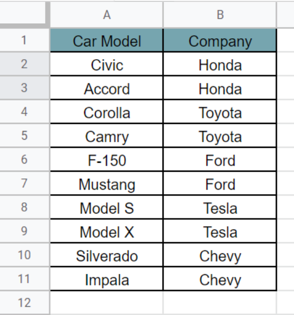
Here we have a dataset, In this dataset, there are the names of car companies and their cars. Now we want to switch the rows into columns and columns into rows, for that purpose we will use Transpose. In this tutorial, we will learn how to Transpose a table in Google Sheets but first let’s take a look at the dataset above.

Method – 1 Using Copy and Paste.

Step – 1 Select the cells.

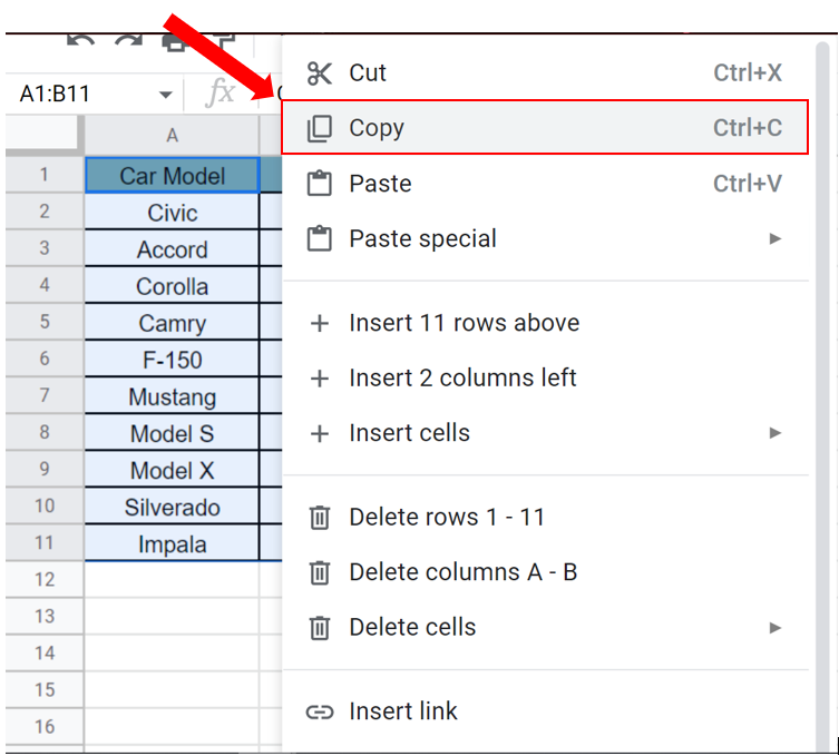
• Select the table you want to transpose.
• Right-click on the selected table, click on the Copy command, or press Ctrl + C to copy the table.
• Then select any empty cell.

Step – 2 Use the Transpose command.

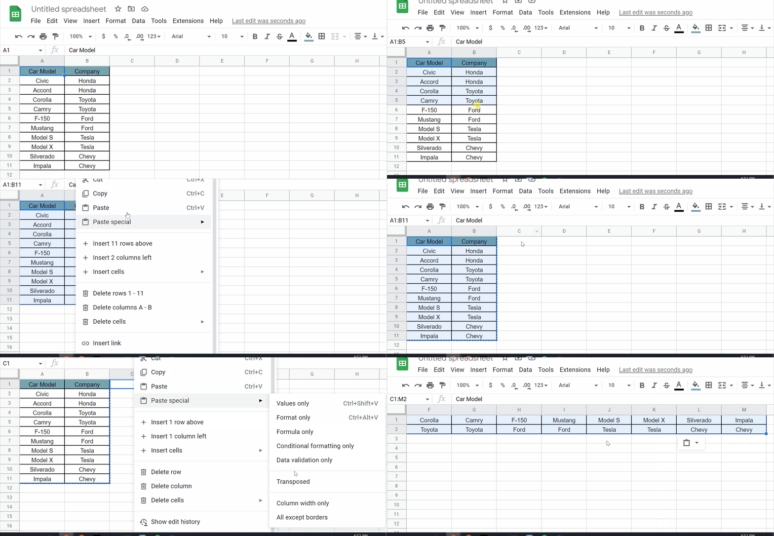
• After selecting the empty cell, right-click on the selected cell.
• In the menu that appears click on Paste Special.
• Then click on the Transpose command that appears.
• The table will be transposed.

Method – 2 Using the Transpose Function.

Step – 1 Select the cell.

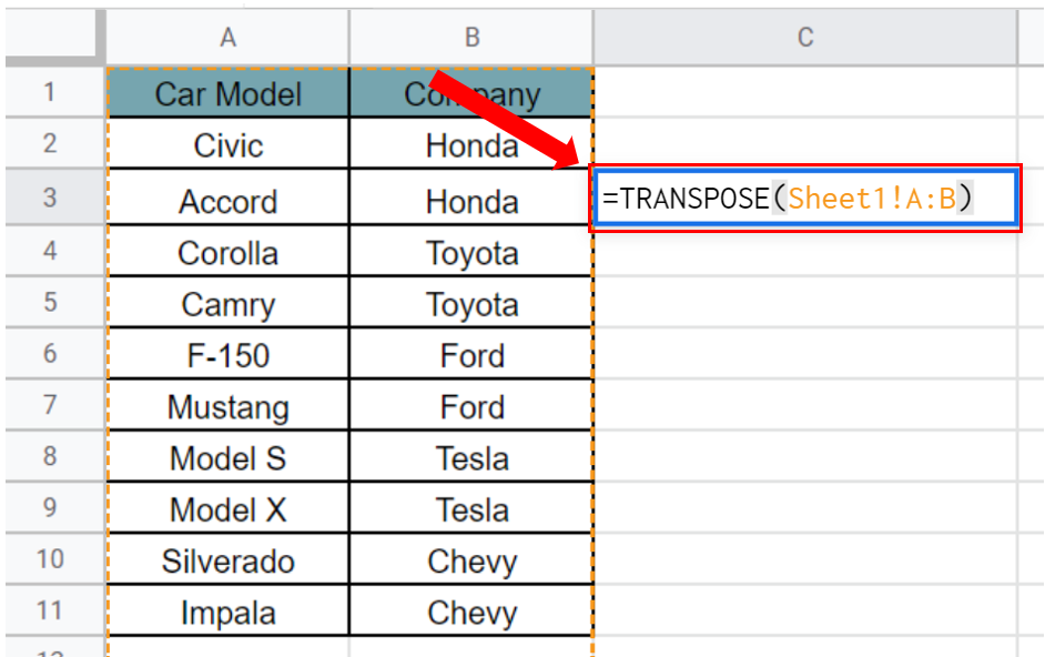
• Select the cell where you want to write the formula.
• The syntax of the formula will be

=TRANSPOSE(Sheet_Number!First_Column:Second_Column)

• In our case the formula will be

=TRANSPOSE(Sheet1!A:B)

Step – 2 Find the values of the rest of the cells.

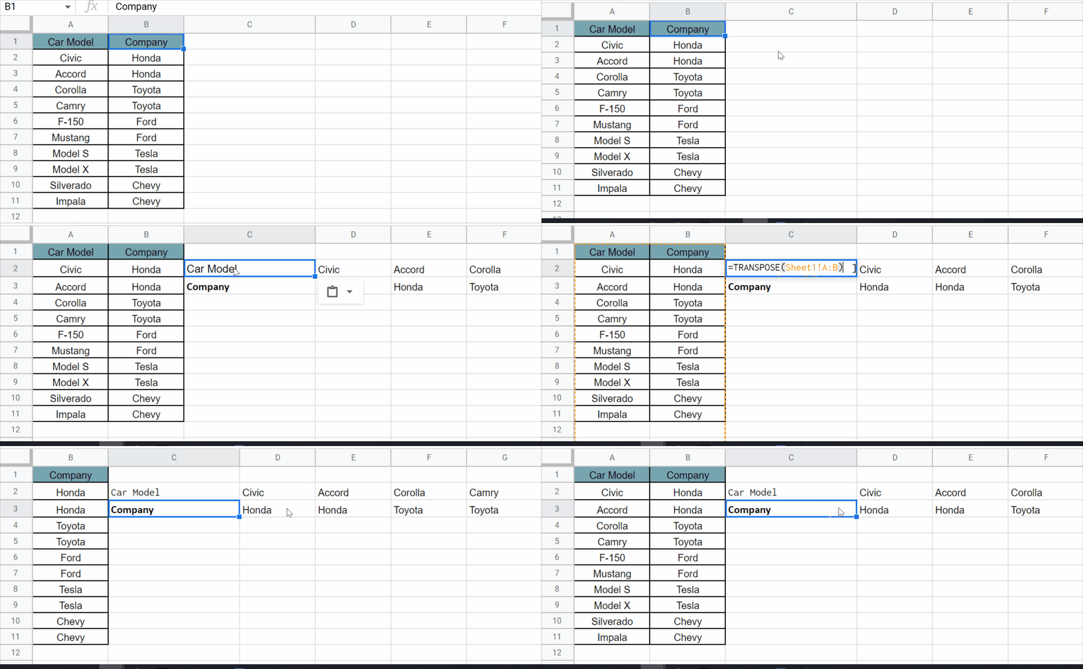
• Click enter on the cell containing the formula.
• The transpose of the table will be created.

Conclusion:

Transposing data in Google Sheets is a simple but powerful tool that can help you analyze and organize your data more effectively. Whether you use the copy and paste method or the TRANSPOSE function, transposing data is an easy way to switch the orientation of your data and gain new insights into your data set.