
How to sum by category in Excel
 By
SpreadCheaters
By
SpreadCheaters
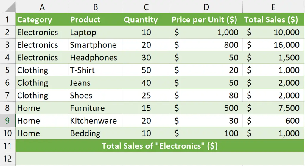
This dataset includes three categories: Electronics, Clothing, and Home. Each category has different products, quantities sold, price per unit, and total sales. We will use this dataset to learn how to sum the values by specific categories.
Understanding the Function and its syntax
SUMIF Function:
The SUMIF function in Excel is used to calculate the sum of values in a range that meets specific criteria. It allows you to sum values based on a single condition.
The syntax for the SUMIF function is as follows:
=SUMIF(range, criteria, [sum_range])
Let’s break down each component of the syntax:
range: This is the range of cells that you want to evaluate against the given criteria. It can be a single column or row, or a combination of both. The values in this range will be checked against the criteria.
criteria: This is the condition or criteria that the values in the range should meet in order to be included in the sum. It can be expressed using comparison operators (such as “=”, “>”, “<“, etc.), text, or logical expressions.
sum_range (optional): This parameter specifies the range of cells from which the corresponding values will be summed if they meet the criteria. It can be the same size as the range parameter or a different range. If the sum_range parameter is omitted, the cells in the range parameter will be summed.
Summing by category in Excel aids in interpreting sales data, leading to better decision-making. By aggregating sales data for each category, it becomes possible to calculate various performance metrics, such as total revenue, average sales per category, or market share.
Step 1 – Select the cell

– Select any empty cell where you wish to calculate the sum of values by category.
– In this cell, we will apply the SUMIF function to get our desired result.
Step 2 – Write and implement the formula

– We wish to calculate the sum of total sales of “Electronics” so, we will write the following formula in the cell:
=SUMIF(A2:A10,”Electronics”,E2:E10)
SUMIF: This is the function name indicating that we want to use the SUMIF function in Excel to perform the calculation.
A2:A10: This is the range of cells in column A that we want to evaluate. In this case, it represents the range where the categories are located.
“Electronics”: This is the criteria or condition that the values in the range A2:A10 should meet. It is enclosed in double quotation marks because it is a text value. In this example, we are looking for cells that contain the text “Electronics” in column A.
E2:E10: This is the range of cells in column E from which the corresponding values will be
summed. It represents the range where the sales values are located.
– Then press Enter and the sum of the sales for the category of “Electronics” will be calculated.
Explanation of Formula used in Step 2:
The formula “=SUMIF(A2:A10,”Electronics”,E2:E10)” calculates the sum of values in column E (E2 to E10) based on a specific condition in column A (A2 to A10). In this case, it adds up the values in column E only if the corresponding cells in column A contain the word “Electronics”. The formula scans each cell in column A, and if it matches the condition, the corresponding value in column E is included in the sum. This formula is useful when you want to find the total of certain values based on a specific criterion or condition in another column.


