How to sort a chart in Excel

Sorting data in Excel enhances data management, analysis, and presentation, leading to improved decision-making and efficiency in various tasks. It allows you to arrange your data logically and identify patterns, trends, and outlines within your data.

In this tutorial, we’ll discuss the most convenient method to sort a chart in Excel.

METHOD – By sorting the input data

In this method, we’ll sort the data source upon which the chart is created.

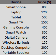
Consider the following data set containing the prices of smart electronic devices of a company.

The following steps should be considered to sort a chart in Excel:

STEP 1 – Select the data set 

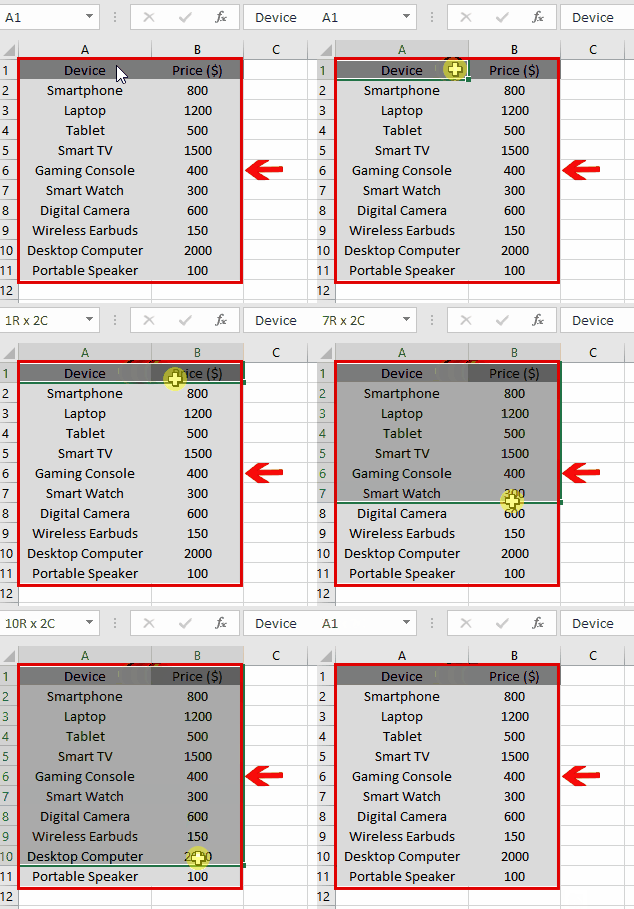
• Move your cursor to the first cell containing data.
• Drag the pointer to the last cell which contains data.
• The whole data set will be selected.

STEP 2 – Locate the charts group

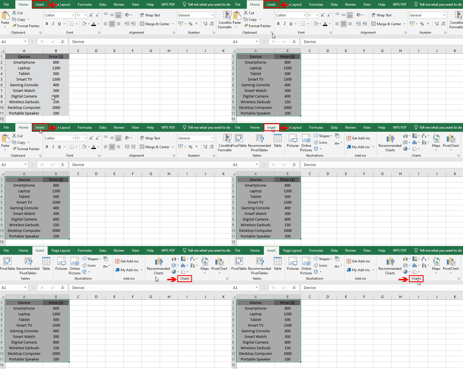
• Go to the Insert tab.
• In the Insert tab, you will find the charts group.

STEP 3 – Insert a bar chart

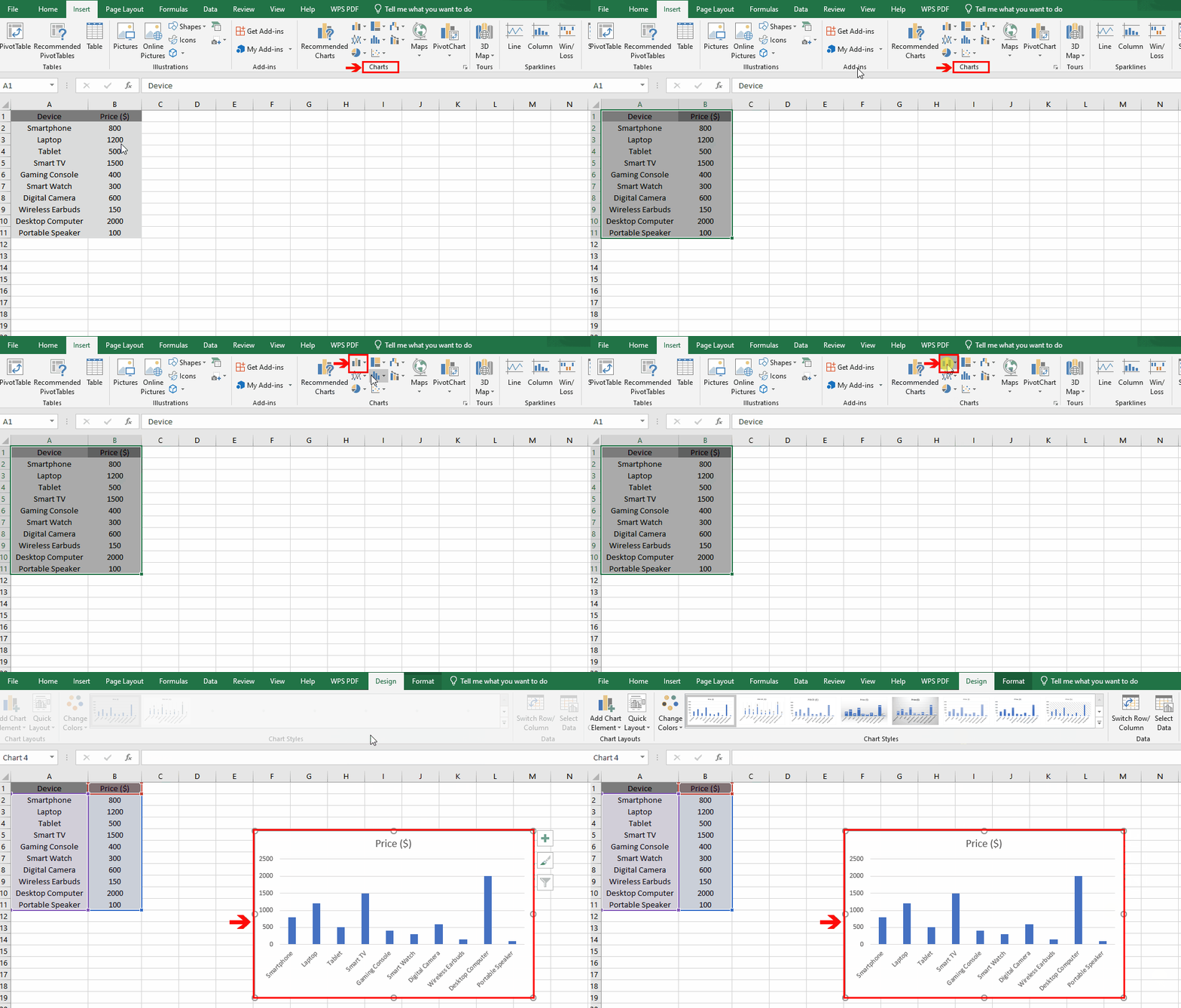
• In the charts group, select the Bar chart option. A drop-down menu will appear.
• In the drop-down menu select the bar chart of your own choice.
• An unsorted bar chart will be inserted in the spreadsheet.

STEP 4 – Select the data source of the vertical axis

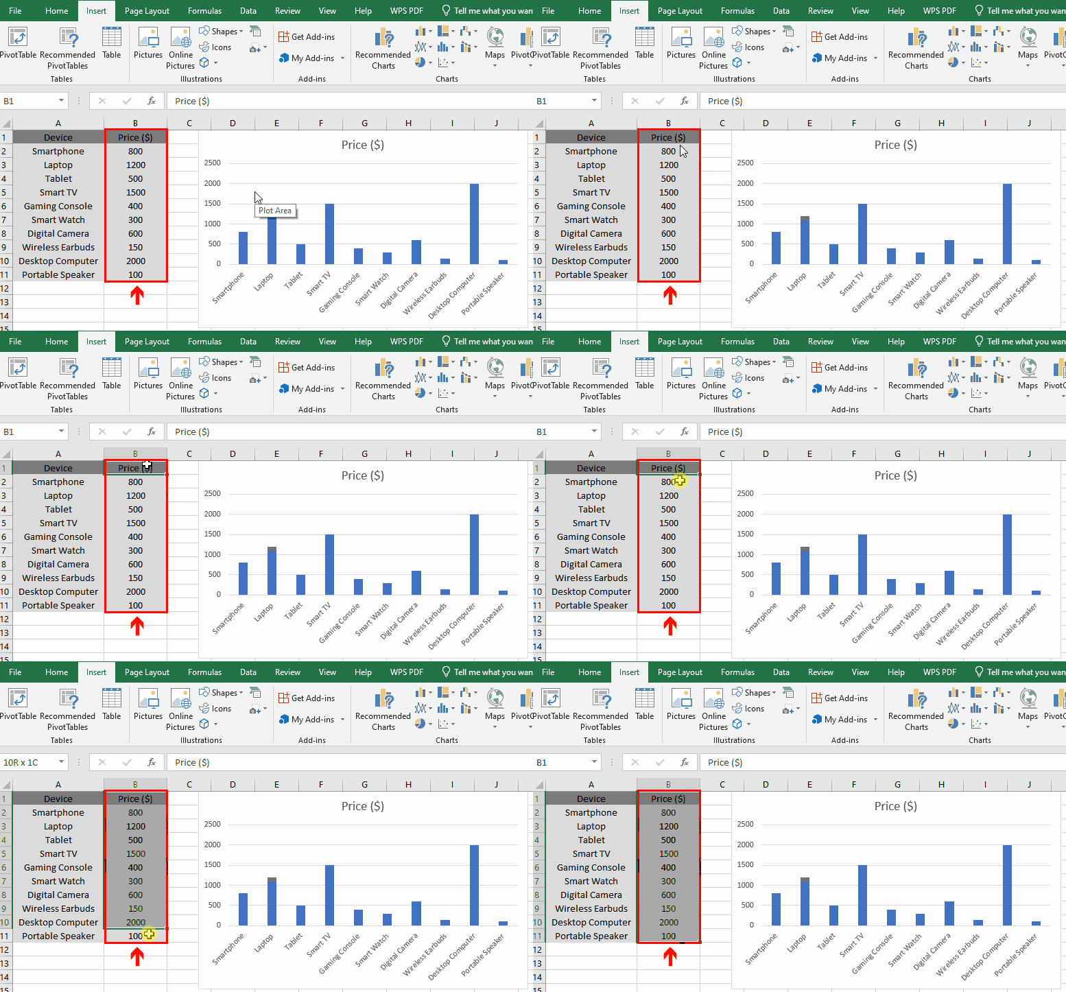
• Move your cursor to the top cell of the column of Price($) in the data set.
• Drag the pointer to the cell containing the price of the last device.
• The data source of the vertical axis will be selected.

STEP 5 – Locate the Sort and Filter group

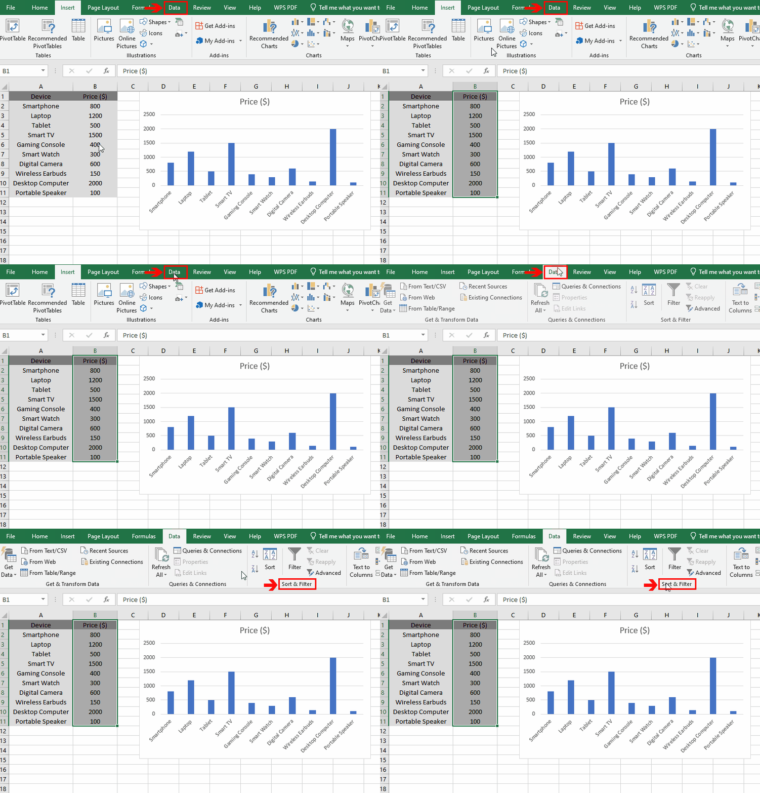
• Go to the Data tab. 
• In the Data tab, you will find the Sort and Filter group.

STEP 6 – Sort the chart

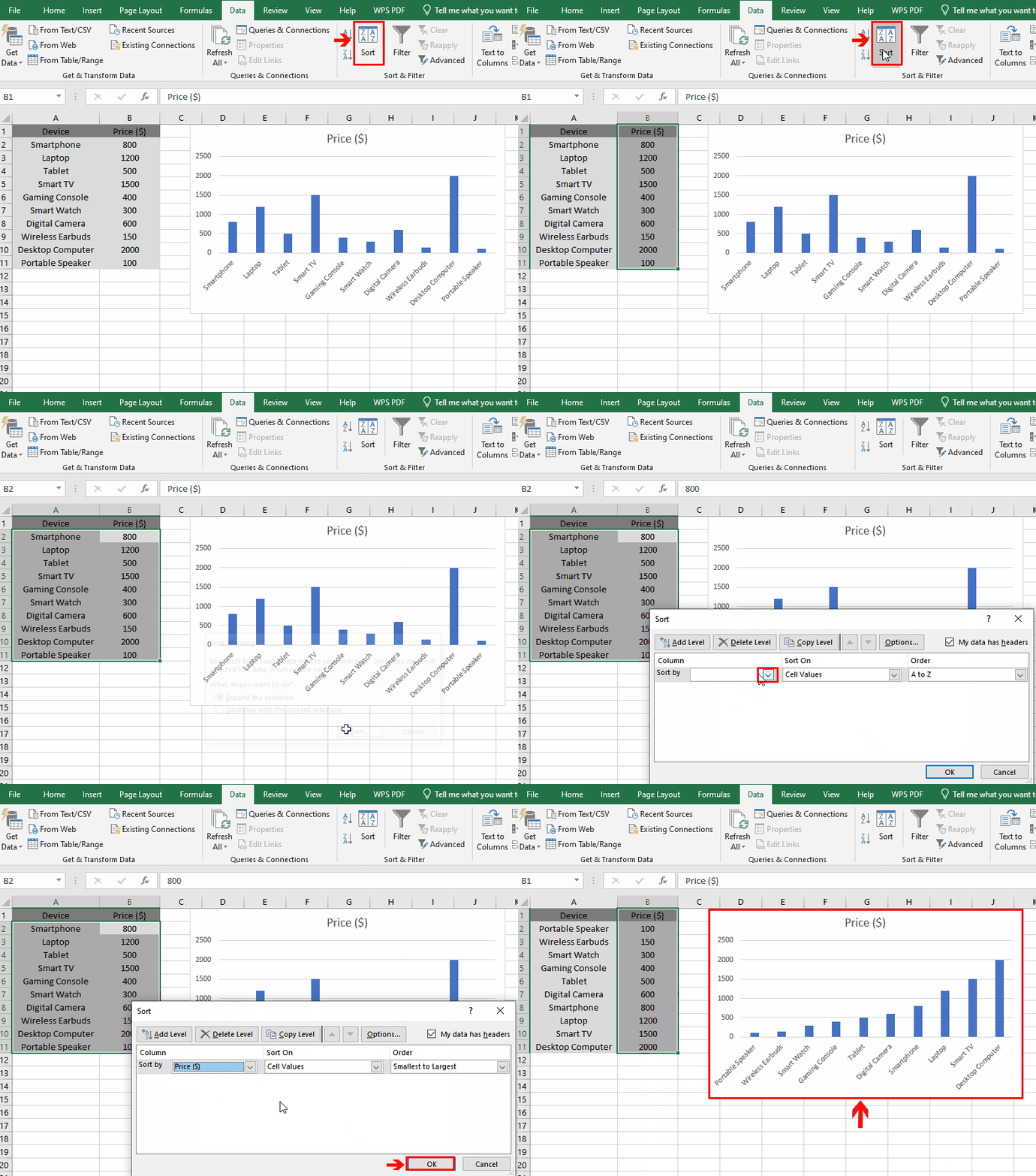
• Select the Sort option in the Sort and Filter group. A dialogue box will appear.
• Click on the Sort option. Another dialogue box will appear.
• Click on the arrow in the Sort by box.
• Select the Price($) option.
• Click on the OK button. Your chart will be sorted.