
How to rearrange columns in a pivot table in Microsoft Excel
 By
SpreadCheaters
By
SpreadCheaters
In this tutorial, we will learn how to rearrange the columns in a pivot table in Microsoft Excel. This can be done by dragging and dropping column headers within the PivotTable Field List, or by using the Move Up and Move Down buttons in the Value Field Settings or Column Labels dialogue boxes.
We have a pivot table that displays the marks obtained by five students in different columns. Our objective is to replace the column that shows Ava’s marks with the first column.
In a Pivot Table in Microsoft Excel, rearranging columns refers to the act of changing the order in which the columns are displayed in the table. It is widely used in Changing the order of columns to better analyze data and improve readability etc.
Step 1 – Click Anywhere on the Pivot Table
– Click anywhere on the pivot table.
– The Pivot Table Analyze tab will appear in the menu bar.
Step 2 – Go to the Pivot Table Analyze Tab
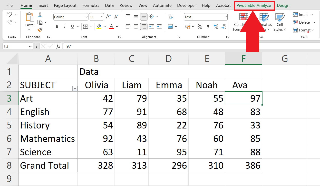
– Go to the Pivot Table Analyze Tab in the menu bar.
Step 3 – Click on the Field List Button
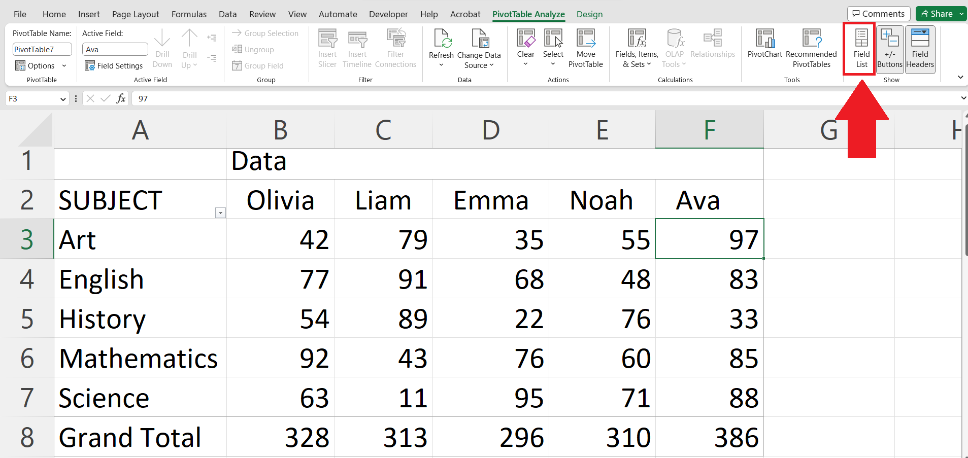
– Click on the Field List button in the Show section.
Step 4 – Hover the Cursor Over the Column Header
– Hover the cursor over the column header of the column you want to move.
Step 5 – Click Hold and Drag the Column Header

– Click and Hold the cursor on the column header and drag it up or down as required.
– Drop the cursor after placing the column header in the desired place.
– The column will be moved in the pivot table.


