How to show the pivot table menu

A pivot table is a tool used in spreadsheet software that makes our work easy. There are several reasons why we need to show the pivot table menu or Pivot Table Field List i.e data summarization, data exploration, Report generation, and Data visualisation. A pivot table menu is a powerful tool that can help you analyse and summarise large datasets in an organised and efficient way. It is mainly used when working with complex data analysis tasks or when we need to generate reports or visualisations based on the data.

To show a Pivot table we can follow these methods:

Method 1 – By Creating a Pivot Table

In this method, we’ll create the Pivot Table first and then show the Pivot Table menu or Field List by following the steps mentioned below.

Step 1 – Locate the Pivot Table option in the Insert Menu

• Open the spreadsheet which contains the data which we need.
• Click on any cell.
• Go to the “Insert” tab at the top right of the spreadsheet.
• Click on the “PivotTable”. A dialog box will open.As shown below;

Step 2 – Define the range and location

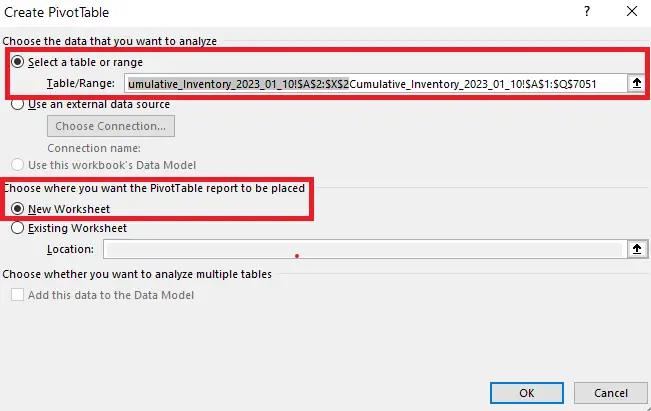
• In the dialog box, define the range of data you want to use. 
• In this case, we proceed with default values. It selects the entire data range by default, e.g “Cumulative_Inventory_2023_01_10!$A$2:$X$2”. ( you can change it as per your requirements ).
• We can also provide the other sources as well, by option given just below.
• Select the location where you want to place the pivot table and choose the options for your pivot table.
• In this case we choose by default settings of New Worksheet. (you can also place this pivot table in the Existing Worksheet option).
• Click “OK” to go to the pivot table. As shown below;

Step 3 – Show Pivot Table Menu or Field List

• Once the Pivot Table is created, the pivot table menu options, which are also called pivot table fields will be visible as the side bar menu. Now we can drag and drop the column headers into the “Rows,” “Columns,” and “Values” areas to customise the pivot table. In the PivotTable pane that appears on the right side of the screen.
• We can also apply filters, sort the data, and perform other actions by using the options in the pane.
• If the pivot table menu is hidden, we can re-enable the pivot table menu by right-clicking on the report area and selecting “show Field list” as shown in the animation below:

Method 2 – By using PivotTable Tools

Once the Pivot table is created we can show or hide the Pivot table menu in excel by using Analyze Option at the top right side of the spreadsheet.

Step 1 – By using Analyze Option under the Pivot table tools

• Open the spreadsheet where the Pivot Table is already created.
• Go to the “Analyze” Option under the Pivot Table Tools.
• After selecting the “Analyze” Option click on the “show” button. A drop down menu will appear.
• From the drop-down menu click on “Field List” to show or hide the PivotTable Fields pane as shown in the animation below:

By using the above two methods we can create, show and hide a pivot table menu in Microsoft Excel.