How to show grand total in Pivot Table

In a pivot table, the grand total represents the sum or total value of a specific data field across all the rows or columns in the table. It provides a comprehensive overview of the aggregated data. 

In this tutorial, we will learn how to show grand total in Pivot Table in Microsoft Excel. Grand total is a useful feature in Microsoft Excel that provides the sum of a specific instantly. Usually, grand total automatically appears when a pivot table is created however if not, then below mentioned are the steps you need to follow. 

Step 1 – Choose the Data 

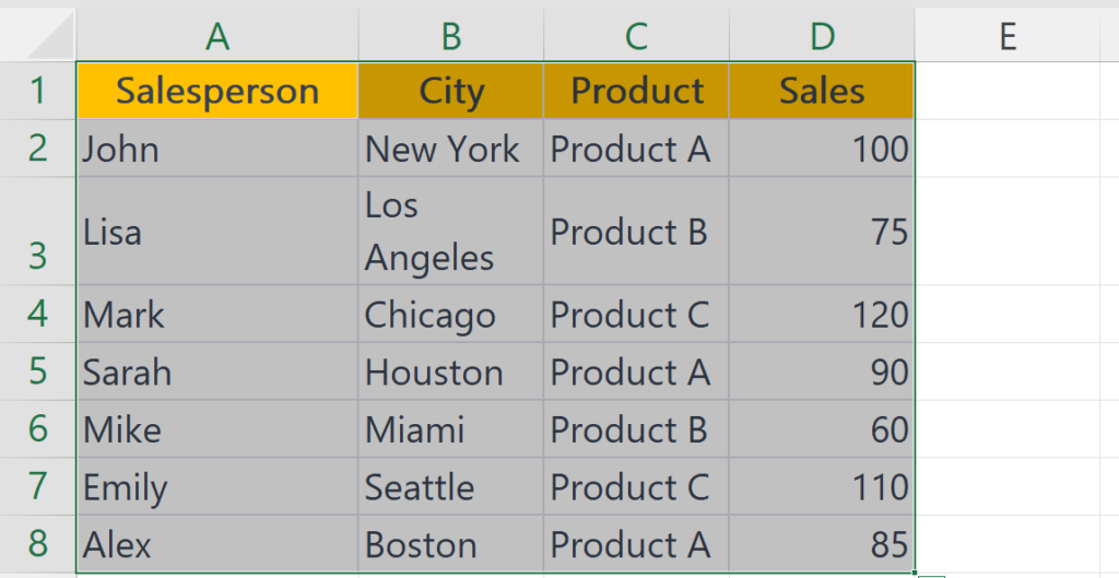
• Choose the data to insert a pivot table. 

Step 2 – Locate the FIle Tab 

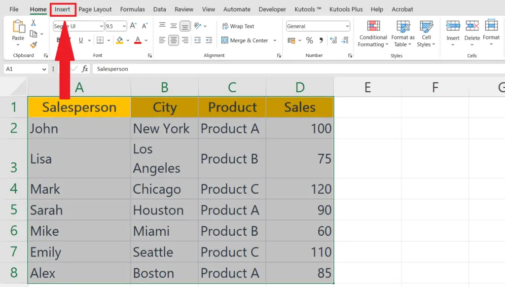
• Locate the File tab in the menu bar. 

Step 3 – Perform a Click on the PivotTable Button  

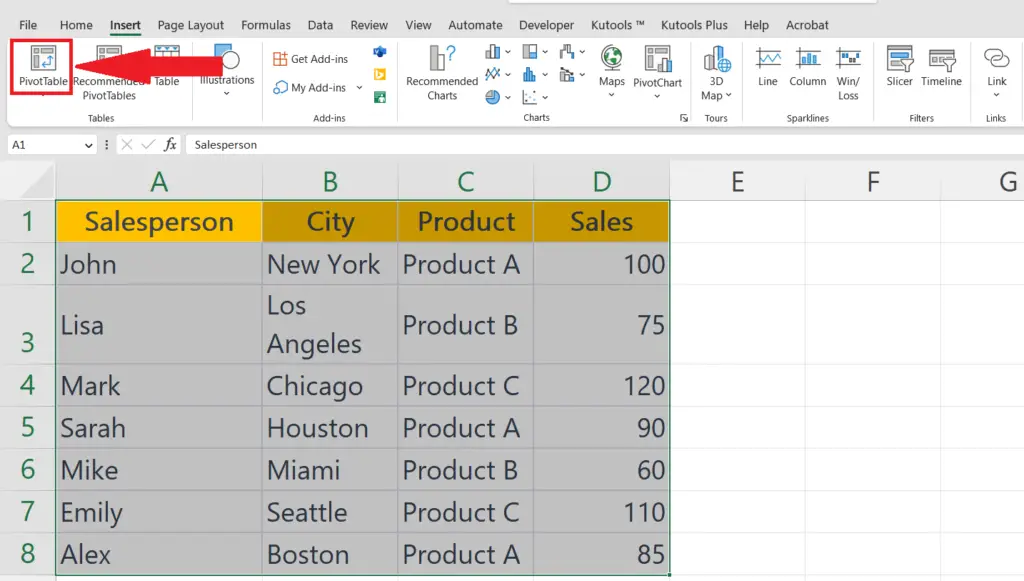
• Perform a click on the PivotTable button at the leftmost of the ribbon. 

Step 4 – Choose the New Worksheet Option 

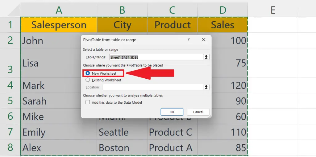
• Choose the New Worksheet option in the dialog box that appear, you may insert the pivot table in the existing sheet if required. 

Step 5 – Select the Field to be Included in the PivotTable 

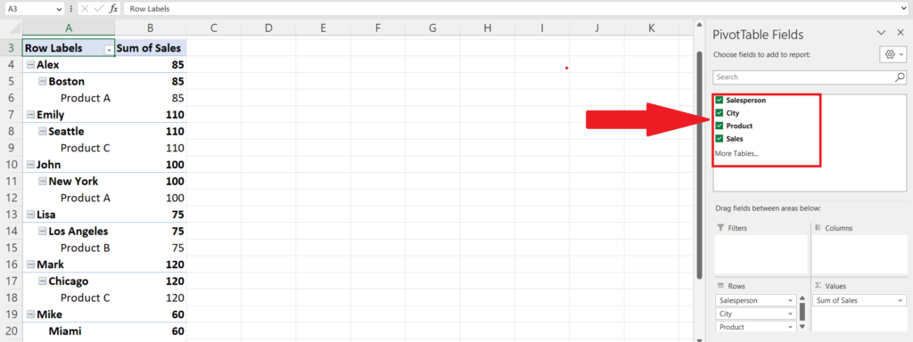
• Select the fields to be included in the PivotTable from the PivotTable Feilds pane at the right of the window. 

Step 6 – Now Click Anywhere on the Pivot Table 

• Perform a click anywhere on the pivot table. 
• This will activate the Design tab. 

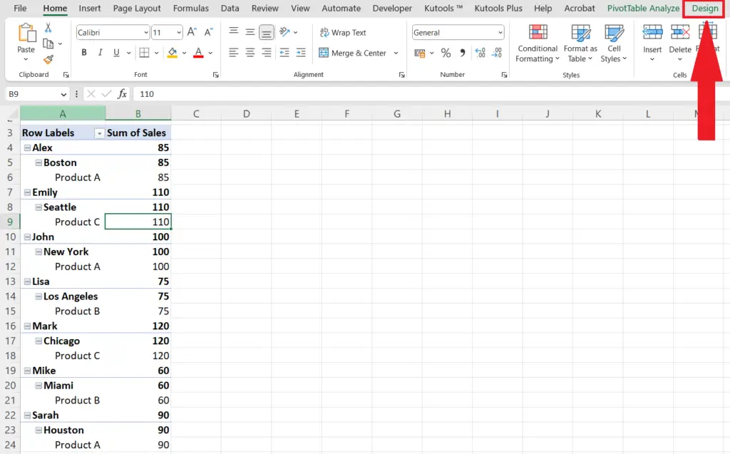
Step 7 – Locate the Design Tab 

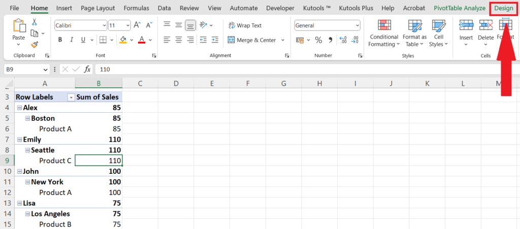
• Locate the Design tab in the menu bar. 

Step 8 – Perform a Click on the Grand Totals Drop-down Arrow 

• Perform a click on the “Grand Totals” drop-down arrow. 

Step 9 – Choose a Suitable Option 

• Choose a suitable option as per your data set. 
• In this case, we will choose the “On for Columns Only” option from the drop-down menu, since our sum of sales for all the products are listed in a column. 
• The Grand Total will appear in the pivot table.