
How to show field headers in PivotTable
 By
SpreadCheaters
By
SpreadCheaters
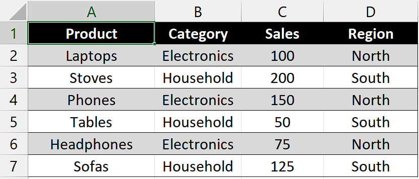
The provided dataset displays the sales figures for various product categories in the given regions which are North and South, with a breakdown of sales in the Electronics and Household sectors. The dataset consists of six rows representing different products: Headphones, Laptops, Phones, Sofas, Stoves, and Tables. Each product category is associated with its corresponding sales amount in the Electronics and Household columns. In today’s tutorial, we will learn how to convert a range to PivotTable and show the Field headers in PivotTable.
Field headers in a PivotTable are the labels that identify the columns or rows representing different data fields or categories. They provide a clear and organized structure to the PivotTable, making it easier to understand and interpret the data. By displaying field headers, the PivotTable becomes more readable and user-friendly. They also allow users to modify the PivotTable layout, rearrange fields, and add or remove categories as needed for analysis.
Step 1 – Select the Range of cells
– Select the range of cells that you want to convert to the PivotTable.
– For example, we have selected the range of cells “A1:D7”.
Step 2 – Convert to PivotTable
– Go to the “Insert” tab on the Excel ribbon, and you’ll find the “PivotTable” button.
– Click on it to open the PivotTable wizard.
– In the PivotTable wizard, the selected range should already be populated in the “Select a table or range” field because we have already chosen the range of cells. Verify that the correct range is displayed and make adjustments if needed.
– Choose where you want the PivotTable to be placed. You have two options:
– New Worksheet: Creates a new worksheet and places the PivotTable there.
– Existing Worksheet: Select a cell in an existing worksheet where you want the PivotTable to be inserted.
– Once you’ve selected your option, click on “OK”.
Step 3 – Design the PivotTable
– You’ll be presented with the PivotTable Field List on the right side of the screen.
– This list contains the column headers from your selected range.
– Drag and drop the fields from the list into the four areas which are Report Filter, Column Labels, Row Labels, and values.
– Choose the field you want to use as a filter for the entire PivotTable. Drag and drop this field from the PivotTable Field List into the “Report Filter” area. For instance, we want to use “Region” as “Report Filter”.
– Select the field you want to be used as column headers in the PivotTable. Drag and drop this field from the PivotTable Field List into the “Column Labels” area. For example, we want to use “Category” as “Column Label”.
– Identify the field you want to be used as row headers in the PivotTable. Drag and drop this field from the PivotTable Field List into the “Row Labels” area. For instance, we want to use “Products” as “Row Label”.
– Specify the field that contains the data to be summarized in the PivotTable. Drag and drop this field from the PivotTable Field List into the “Values” area. We entered the “Sales” field in the “Values” area.
– Once you’ve dropped everything into the four areas given then your PivotTable will automatically be generated.
Step 4 – Show the Field Headers
– As we can see, our PivotTable isn’t showing Field Headers.
– To enable them, navigate to the “PivotTable” Analyze tab.
– Locate the “Field Headers” command button under the “Show” group.
– Click on the “Field Headers” command button and your Field Headers will show up.
Step 5 – Modify the names of Field Headers
– The Field Headers are named “Row Labels” and “Column Labels” by default but if you want to change their name according to your preference then, select the cell containing “Row Labels” and “Column Labels”.
– Then, click the Formula Bar and rename them according to your desire.
– For instance, we have named “Row Labels” as “Products” and “Column Labels” as “Categories”.
– Alternatively, you can press “Alt Key” and press “J key” with the “T key” to open the “PivotTable” Analyze tab.
– Then, press the “H key” to show the Field Headers.


