
How to add data to a Pivot Table in Microsoft Excel
 By
SpreadCheaters
By
SpreadCheaters
In this tutorial we will learn how to add data in a Pivot Table in Microsoft Excel. It’s a straightforward process to include additional information in a pivot table. By accessing the “Change Data Source” option in the “PivotTable Analyze” tab, we can easily append new data to the existing table. This feature allows us to quickly update and modify our pivot table to reflect the latest data changes, without having to recreate the entire table from scratch.
We currently have a pivot table displaying the sales of products for the first four months of a data set. The plan is to include the sales for two more products in the pivot table.
A Pivot table is a powerful tool in spreadsheet software that allows users to quickly summarize and analyze large amounts of data in a flexible and interactive way. It works by taking a dataset and allowing the user to “pivot” or reorganize the data in various ways, such as by grouping, filtering, or sorting. This makes it easy to see patterns, trends, and relationships within the data.
Step 1 – Click Anywhere on the Pivot Table
– Click anywhere on the Pivot table.
– “PivotTable Analyze” tab will appear in the menu bar.
Step 2 – Go to the PivotTable Analyze Tab
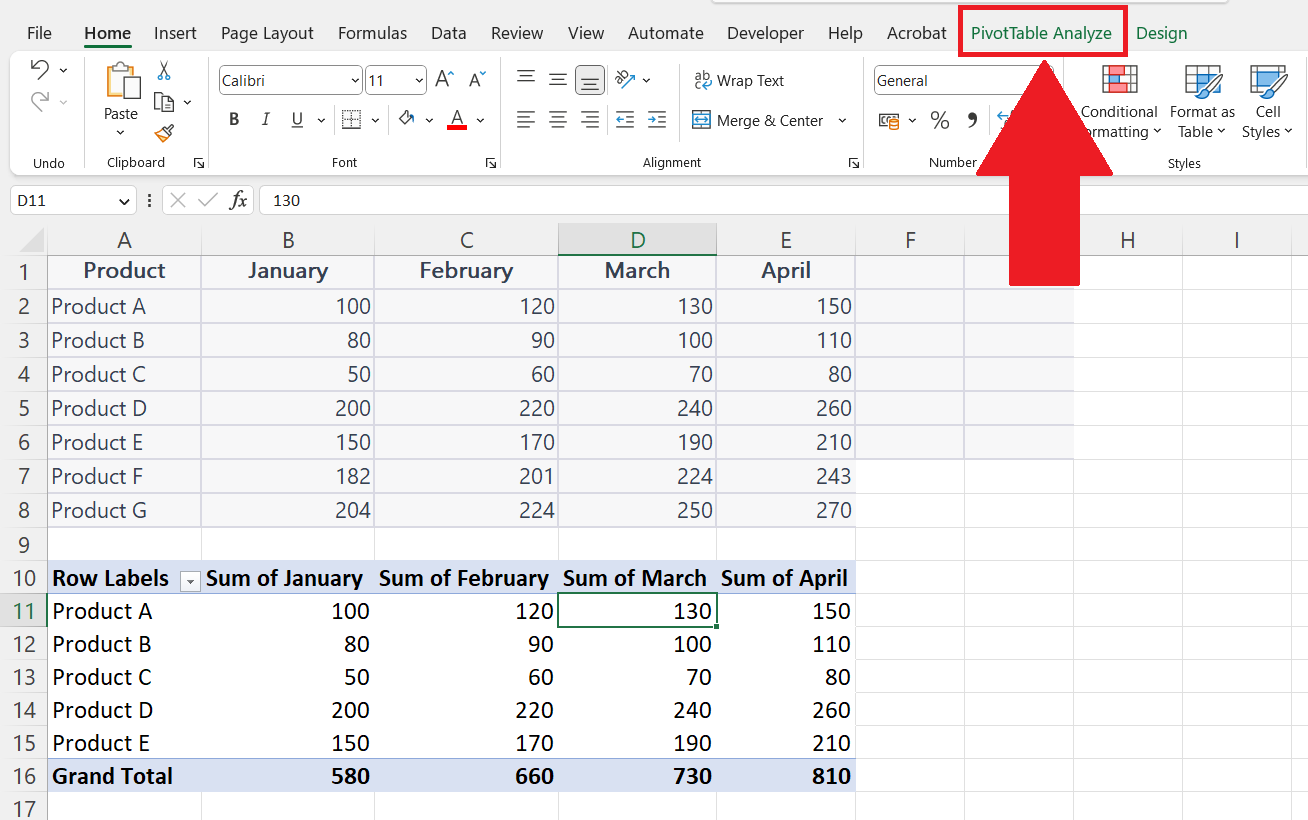
– Go to the Pivot Table Analyze Tab in the menu bar.
Step 3 – Click on Change Data Source Button
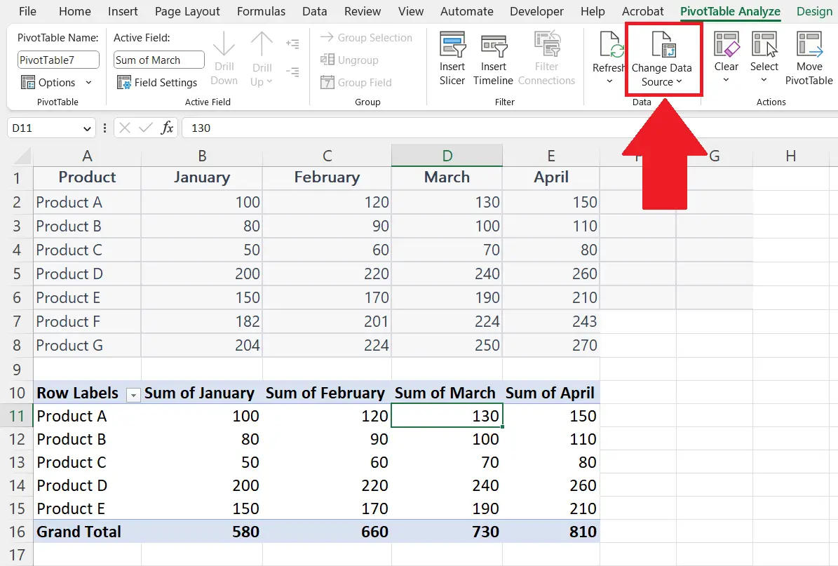
– Click on the Change Data Source button in the Data section.
– Change PivotTable Data Source dialog box will appear.
Step 4 – Select the Range of Data
– Select the range of data including the additional data to be added in the pivot table.
– You may enter the range manually or use the “Handle Select” and “Drag and Drop” method in the Select a table or range option.
Step 5 – Click on OK

– Click on OK in the PivotTable Data Source dialog box.


