How to show an Intersection point in a Microsoft Excel graph

In Excel, showing the intersection point on a graph refers to displaying the coordinates where two or more plotted lines or curves intersect. This feature is particularly useful when analyzing data and identifying the exact point of intersection between different variables or trends. 

In this tutorial, we will learn how to show an Intersection point in a Microsoft Excel graph. In Microsoft Excel, we can simply identify the intersection point by utilizing the scatter chart with a smooth line. 

Currently, we have a line chart, and our objective is to display the point where the line intersects with another line that has its data points specified within the sheet. 

Step 1 – Select the Range of the cell 

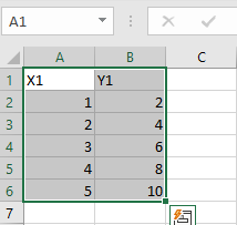
• First, select the range of the cell of the first dataset 

Step 2 – Go to the Insert  

• Now go to the Insert tab and select the option Insert Scatter from the Chart group options 

Step 3 – Click on the option Scatter with Smooth line 

• Select the option “Scatter with Smooth line” from the Scatter group options and the graph of your first data set will appear on the sheet. 

Step 4 – Select the option, Select Data 

• Now right-click on the graph and select the option of Select Data and a dialog box will open 

Step 5 – Perform a Click on the Add Button 

• Afterward, click on the Add option and a new Dialog box will open 

Step 6 – Select the range of X values 

• Now select the range of X Values of the second data set 

Step 7 – Select the range of Y values  

• Now select the range of Y values of The second Data Set 

Step 8 – Perform a Click on Ok 

• Now perform a click on the Ok of the Dialog Box and then click on the OK of another Dialog Box after that graph of the data set with intersection points will appear. 

Step 9 – Identify the Intersection Point 

• To identify the intersection point we can add “Data Callouts”. 
• For this, select the chart. 
• Click on the “Chart Elements” green plus button located at the upper right corner of the chart. 

• Perform a click on the “Data Labels” option and select “Data Callout”.