
How to select random cells in Excel
 By
SpreadCheaters
By
SpreadCheaters
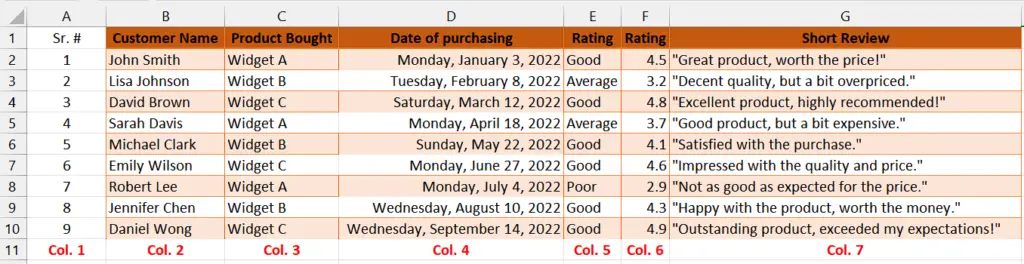
The given dataset consists of customer reviews for different widgets purchased on various dates. Each row represents a customer’s name, the product they bought, the date of purchase, a rating, a numerical rating value, and a short review describing their experience with the product. We need to select random rows to see random reviews of products by people.
Understanding the Functions and their syntax
VLOOKUP Function:
The VLOOKUP function in Excel is used to search for a value in the leftmost column of a table and retrieve a corresponding value from a specified column within that table. The function stands for “Vertical Lookup” because it searches vertically (top to bottom) in a table.
The syntax for the VLOOKUP function is as follows:
=VLOOKUP(lookup_value,table_range,col_index_num,[range_lookup)
lookup_value: This is the value you want to search for in the leftmost column of the table. It can be a specific value, a cell reference, or a formula that evaluates to a value.
table_range: This is the range of cells that represents the table from which you want to retrieve data. The leftmost column of the table should contain the lookup values and the desired data should be located in columns to the right of the lookup column.
col_index_num: This is the column number in the table from which you want to retrieve the result. For example, if you want to retrieve data from the second column of the table, you would use the number 2.
range_lookup: This parameter is optional. It determines whether you want an exact match or an approximate match for the lookup value. If set to TRUE (or omitted), the function will perform an approximate match using the nearest smaller value. If set to FALSE, the function will only return an exact match.
RANDBETWEEN Function:
The RANDBETWEEN function in Excel is used to generate a random integer between two specified values, inclusively. It returns a random whole number within the given range.
The syntax for the RANDBETWEEN function is as follows:
=RANDBETWEEN(bottom, top)
Let’s break down each parameter:
bottom: This is the lower boundary or minimum value of the range from which you want to generate a random number.
top: This is the upper boundary or maximum value of the range from which you want to generate a random number.
In Excel, selecting random rows in Excel provides flexibility in working with data, allowing you to perform statistical analysis, data exploration, testing, and simulations effectively. It helps ensure unbiased representation and adds an element of randomness to your data processing tasks.
Step 1 – Assign Serial number to all rows
– First of all, assign serial numbers to all rows if they don’t have serial numbers already.
– Without assigning these serial numbers, we cannot move further to select random rows.
Step 2 – Select the cell for RANDBETWEEN Function
– Select any vacant cell in which our serial numbers will be randomized.
– In this cell, we will apply the RAND Function.
Step 3 – Use RANDBETWEEN Function in the selected cell

– Start by entering the equal sign (=) to initiate the formula.
– Next, type “RANDBETWEEN” and select the RANDBETWEEN function by pressing the tab button.
– In the first parameter, specify the bottom value of the range from which you want to generate a random number. In this case, it is 1 which is basically representing the first row.
– Insert a comma (“,”) to separate the parameters.
– In the second parameter, specify the top value of the range from which you want to generate a random number. In this case, it is 9 which is basically representing the last row.
– After specifying all the parameters, insert a closing parenthesis “)” to close the formula.
– After following all the steps above, the final formula would look like this:
=RANDBETWEEN(1,9)
– Then press Enter and a random number between 1 and 9.
Step 4 – Select the number of rows to randomize

– Use the fill handle and drag down the formula to desired number of cells which will basically specify how many rows we want to randomize.
– For instance, we have implemented the formula to only 3 cells in total.
Step 5 – Select the cell for VLOOKUP Function
– Select any vacant cell in which we will apply the VLOOKUP Function.
Step 6 – Write the formula using VLOOKUP Function
– Start by entering the equal sign (=) to initiate the formula.
– Next, type “VLOOKUP” to specify the VLOOKUP function.
– After typing “VLOOKUP,” insert an open parenthesis “(” to start specifying the parameters.
– In the first parameter, specify the search key, which is the value you want to look up. In this case, it is the value in cell A15.
– Insert a comma (“,”) to separate the parameters.
– In the second parameter, specify the range of cells that contains the data you want to search in. In this case, it is the range $A$2:$G$10, which means the lookup range spans from column A to column G and rows 2 to 10. Add these dollar signs before and between the cell name to lock this parameter.
– Insert another comma (,) to separate the parameters.
– In the third parameter, specify the column index number from which you want to retrieve the corresponding value. In this case, it is 2, indicating that you want to retrieve the value from the second column of the lookup range and we have written Col.2 to indicate column 2 as well.
– After specifying all the parameters, insert a closing parenthesis “)” to close the formula.
-After following all the steps above, the final formula would look like this:
=VLOOKUP(A15,$A$2:$G$10,2)
-Then, press Enter and the result would appear in the cell.
Step 7 – Modify the formula for all columns in the row
– Write the same formula in the adjacent cell but change the last parameter value according to the column number. For example, we will change the value in “index_num” to 3 for column 3.
– Repeat this step for all columns in the row.
Step 8 – Apply the above formulae to desired number of rows
– Select the whole row in which we have implemented the formulae.
– Then, use the fill handle to apply the above formulae to desired number of rows that we want to randomize.
Step 9 – Randomize the rows by shortcut key
– To select random rows, press the “F9 key” on your keyboard.
– As soon as you use this shortcut, the functions that we applied will select random rows from our dataset.


