
How to select a random cell in Excel
 By
SpreadCheaters
By
SpreadCheaters
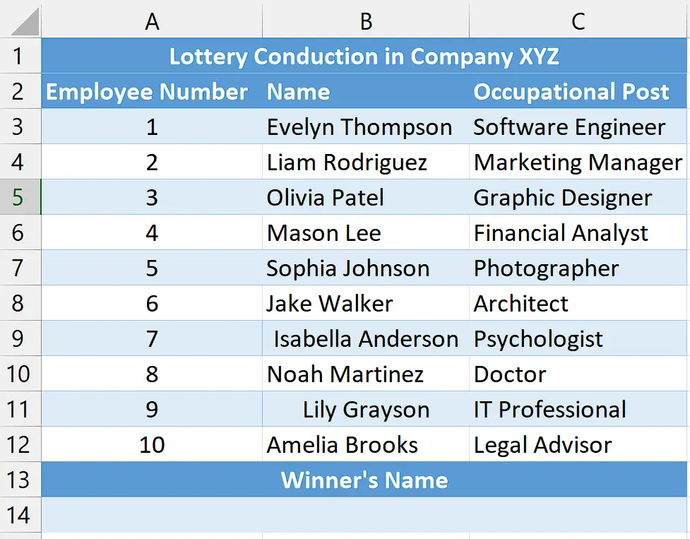
An instance where you might require selecting a random cell in Excel is when facilitating a lottery or a random drawing. Suppose you are arranging a company function and wish to choose a prize winner from a list of employees. In such a case, you can utilize Excel to record the names of employees in one column and assign each name a distinct number in the adjacent column and then find the first three winners by selecting a random cell.
Understanding the Functions and their syntax
CHOOSE Function:
The CHOOSE function in Excel allows you to select a value from a list of values based on a specified index number. Its syntax is as follows:
=CHOOSE(index_num, value1, value2, …)
index_num – This is the index number that specifies which value to select from the list. It must be a positive whole number.
value1, value2, … – These are the values or cells that form the list from which the function will choose. You can provide up to 254 values.
RANDBETWEEN Function:
The RANDBETWEEN function in Excel generates a random integer between two specified numbers. Its syntax is as follows:
=RANDBETWEEN(bottom, top)
bottom: This is the lower boundary or minimum value for the random number generation.
top: This is the upper boundary or maximum value for the random number generation.
The RANDBETWEEN function will return a random whole number that falls between the bottom and top values, inclusive of both boundaries. Each time the worksheet is recalculated or the function is re-evaluated, a new random number within the specified range will be generated.
Selecting a random cell in Excel is beneficial for introducing randomness and variability into analysis, sampling, or data manipulation tasks. It enables randomized data sampling, allowing you to extract a representative subset from a larger dataset. Additionally, random cell selection is useful in experiments or randomized assignments to allocate participants or data points into different groups or conditions.
Step 1 – Select the cell
– Select an empty cell where you would like to obtain the value of a random cell.
– In this cell, we will apply the RANDBETWEEN and CHOOSE Functions to select a random cell.
Step 2 – Write and implement the Formula
– After selecting the cell, write the following formula in the cell.
=CHOOSE(RANDBETWEEN(1,10),B3,B4,B5,B6,B7,B8,B9,B10,B11,B12)
Where,
RANDBETWEEN(1,10): This function generates a random number between 1 and 10, inclusive. The range (1 to 10) represents the number of choices available.
CHOOSE(): This function selects an item from a list based on a given index. In this case, the index is the random number generated by RANDBETWEEN(), and the list consists of the range of cells (B3 to B12) containing the names of the potential lottery winners.
B3, B4, B5, B6, B7, B8, B9, B10, B11, B12: These are the cells containing the names of the potential lottery winners. The CHOOSE() function will choose one of these names based on the random number generated.
– Once you’ve entered the formula in the cell, press Enter button on the keyboard to implement the formula in the cell.
– This will generate a random name which will be the lottery winner.
– To select additional random cells and announce two more winners, press the “F9” key.
Explanation of the formula used in Step 2
The formula =CHOOSE(RANDBETWEEN(1,10),B3,B4,B5,B6,B7,B8,B9,B10,B11,B12) is designed to select a random cell from a list in Excel. By using the RANDBETWEEN(1,10) function, a random number between 1 and 10 is generated, representing the index of the desired cell. The CHOOSE() function then uses this random number to select the corresponding item from the list of cells, which includes B3, B4, B5, B6, B7, B8, B9, B10, B11, and B12. With each recalculation or refresh, a new random number is generated, allowing the formula to pick a different cell from the list, providing a random selection each time.


