How to Randomize a Column in Microsoft Excel

Randomizing a column in Excel means changing the order of the cells in the column in a random manner. This is useful when you want to create a random order of data, such as when selecting a random sample from a larger data set or shuffling a list of items.

In this tutorial, we will learn how to Randomize a column in Microsoft Excel. There are various techniques available in Microsoft Excel to randomize a column. One of the popular ways is to use a combined formula of SORTBY, RANDARRAY, and COUNTA functions, which helps to shuffle the order of cells in a column randomly. 

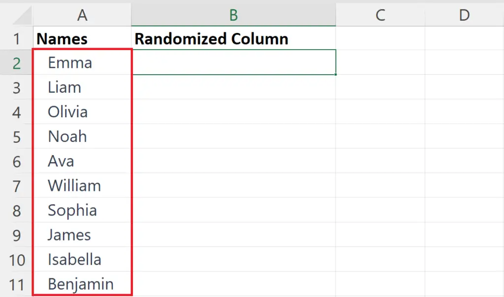
We have column A in the dataset containing a list of participants for competition and our goal is to randomize the order of this list.

Method 1: Using a Combination of SORTBY, RANDARRAY, and COUNTA Functions

The syntax of the combined formula for randomizing a column becomes:

                                 SORTBY(range,RANDARRAY(COUNTA(range)))

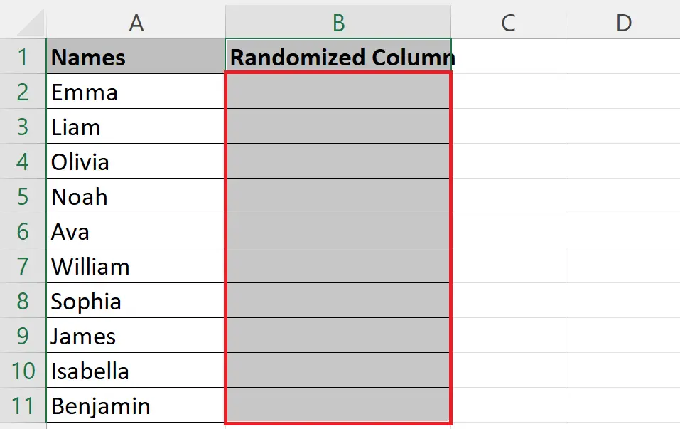
Step 1 – Select a Blank Cell 

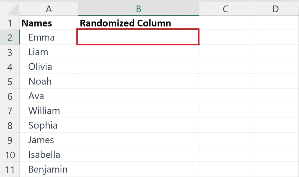
• Select a cell in the column where you want to print the randomized column.

Step 2 – Place an Equals Sign

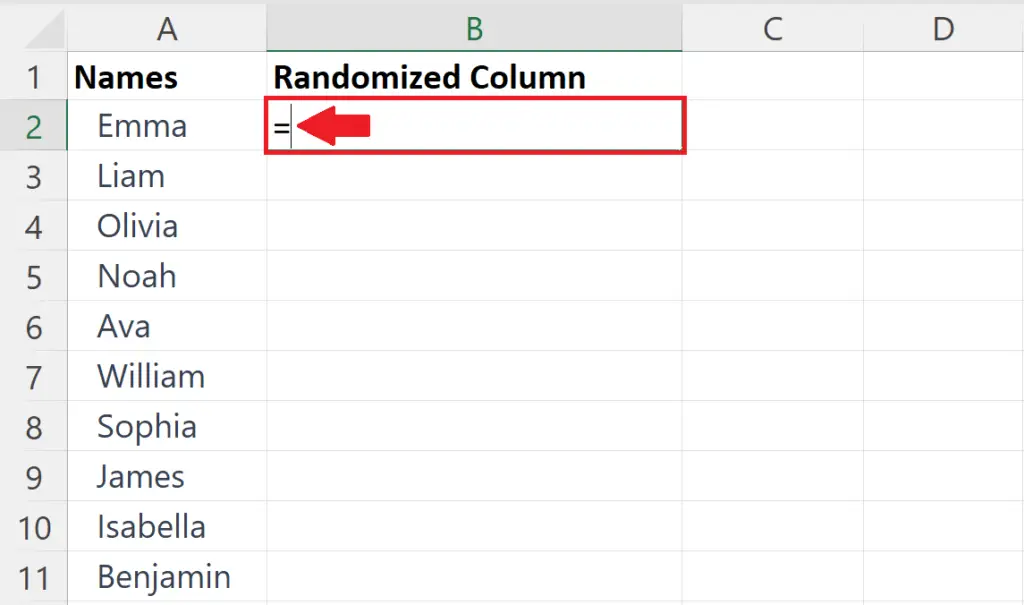
• Place an Equals Sign in the blank cell.

Step 3 – Enter the SORTBY Function 

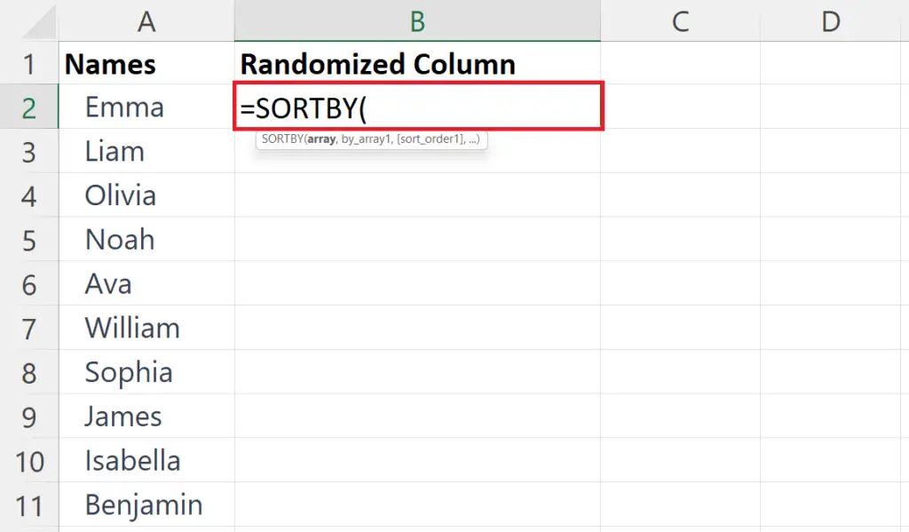
• Enter the SORTBY function right after the equals sign in the cell.
• The SORTBY function takes two arguments i.e. the range to be sorted and the array to use as the sort key.
• Open parentheses.

Step 4 – Enter the Range of Column

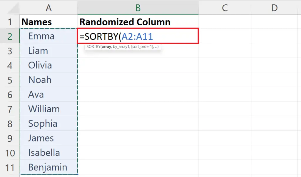
• Enter the range of the Column to be randomized.

Step 5 – Enter the RANDARRAY Function

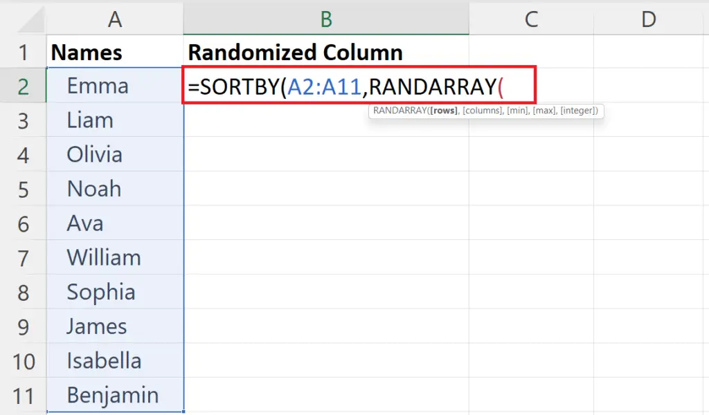
• Enter the RANDARRAY function after placing a comma ( , )  after the range.
• RANDARRAY() creates an array of random numbers with the same length as the number of non-blank cells in the range.
• Open parenthesis.

Step 6 – Enter COUNTA Function

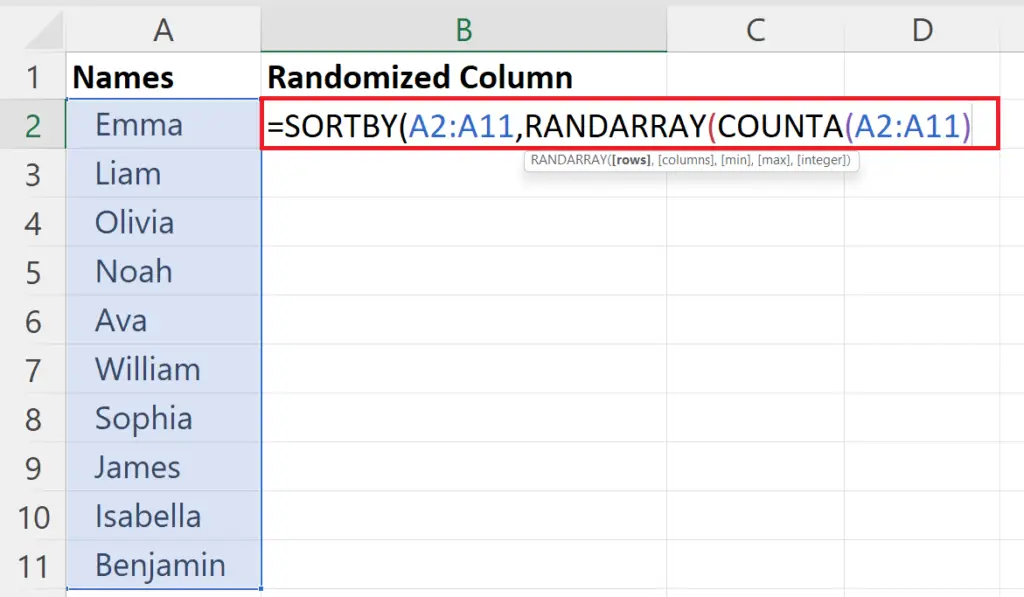
• Nest the COUNTA function in the RANDARRAY function and enter the column range to be customized as its argument i.e. COUNTA(range).
• The COUNTA function counts the number of non-blank cells in the range.
• Close the parenthesis of the COUNTA function.

Step 7 – Close the Parenthesis of the RANDARRAY Function and the SORTBY function

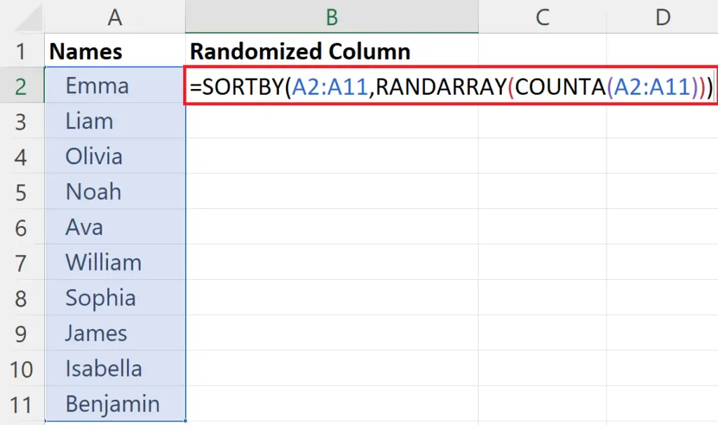
• Close the Parenthesis of the RANDARRAY function.
• Close the Parenthesis of the SORTBY function.

Step 8 – Press the Enter Key

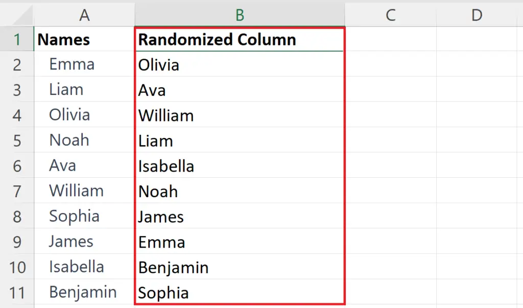
• Press the Enter key.
• The randomized column will be printed in the selected column.

Method 2: Using the RAND() Function

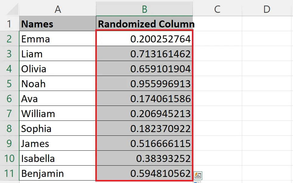
Step 1 – Select a Helper Column

• Select a helper column.

Step 2 – Enter RAND() Function

• Enter the RAND() function in the first cell of the column.
• Press the Enter key.

Step 3 – Use Autofill to Apply RAND() Function

• Use Autofill to apply RAND() function across the column.

Step 4 – Now Select the Helper Column

• Select the Helper column.

Step 5 – Go to the Data Tab and Click on a Sort Option

• Go to the Data tab.
• Click on any of the sort options in the Sort & Filter section i.e. Sort A to Z.

Step 6 – Select the Expand Selection Option

• Select the Expand the selection option in the dialog box that appears.
• Click on OK.
• The column containing the names will be randomized.