How to remove spaces between numbers in Excel

In Excel, you may need to remove extra spaces between numbers when you’re working with numerical data such as performing calculations or creating charts. Extra spaces can interfere with the accuracy of your results. For example, if you have a column of numbers with varying spaces, it may be challenging to perform mathematical operations or apply functions correctly.

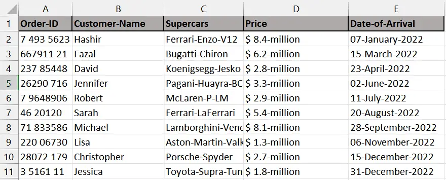
The dataset provided below contains information related to 10 orders of supercars in the year 2022. Each order is identified by an Order ID associated with it. The dataset includes details such as the Customer Name, Supercar model, Price (in millions), and Date of Arrival. There are unnecessary spaces between the numbers present in Order IDs and we need to eliminate the spaces between numbers in the Order ID of each order. One might think here that the good old TRIM function can come to save your life but unfortunately, the TRIM function works only on the text values and it doesn’t work for numeric values.

The following are 2 methods to perform our task:

Method 1 – By using Find and Replace tool

Step 1 – Selecting the Range of cells

• Select the range of cells in which numbers with spaces are present.
• We selected this range because we want to remove spaces from numbers only present in these cells. If we do not select any particular range then it will remove spaces from all cells in the sheet.

Step 2 – Open the Find and Replace tool

• Look for the “Find and Replace“ function.
• In Microsoft Excel, you can find it under the “Home” menu. It is usually represented by a magnifying glass icon or a binoculars icon.
• Click on the “Replace” option to open the tool.
• Alternatively, you can press “Ctrl + H” on your keyboard to open the Find and Replace dialog box.

Step 3 – Removing the spaces

• After following the above step, add a space in the “Find what” option.
• Then, leave the “Replace with” option empty.
• Now, click on the “Replace All” option and all spaces will be removed.
• Click on the OK option on the dialogue box that has appeared.
• Then, close the dialogue box.

Method 2 – By using the SUBSTITUTE Function

Step 1 – Selecting the cell

• Firstly, select any empty cell in which we want to get the numbers without spaces. For example, it is cell B2 in our case.
• In this selected cell, we will apply the SUBSTITUTE Function to remove spaces.

Step 2 – Writing and implementing the formula

• After the cell is selected, press the = (equal sign) on your keyboard.
• Then, write and select the SUBSTITUTE Function.
• Select or write the name of the cell where the original text is located. In this case, it is cell A2.
• Then, enter a comma (,) which will move you to the next parameter which is “old_text”.
• This is the argument within the SUBSTITUTE function and represents the character or text you want to replace. In this case, it is a space character (” “).
• After that, enter a comma (,) and you will move to the next argument which is “new_text”.
• This is the next argument within the SUBSTITUTE function and represents the character or text you want to replace the original character with. In this case, it is an empty string (“”) which means you want to remove the space character.
• Then, add a closing parenthesis and your formula would look like this,

=SUBSTITUTE(A2,” “,“”)

• Now, press Enter and all the spaces from the number in the cell A2 will be removed.

Step 3 – Applying the formula to the whole range

• Select the cell that contains the formula result. For example, in our case, it is cell B2.
• Move your cursor to the bottom-right corner of the selected cell. The cursor will change to a “+” shape, which is known as the fill handle.
• Double-click on the fill handle. Excel will automatically apply the formula to the entire range based on the pattern it detects.