How to remove non-duplicates in Excel

Removing non-duplicate values in Excel can be helpful in several situations such as: Filtering data, simplifying data, and reducing file size. Overall, removing non-duplicate values in Excel can help to streamline the data and make it easier to work with.

The methods to remove non-duplicate values are as under:

Method 1 – Using the IF and COUNTIF formula

To remove non-duplicate values and keep only duplicates you can follow these steps. We will use a combination of IF and COUNTIF functions.

Step 1 – Apply the formula to the available data

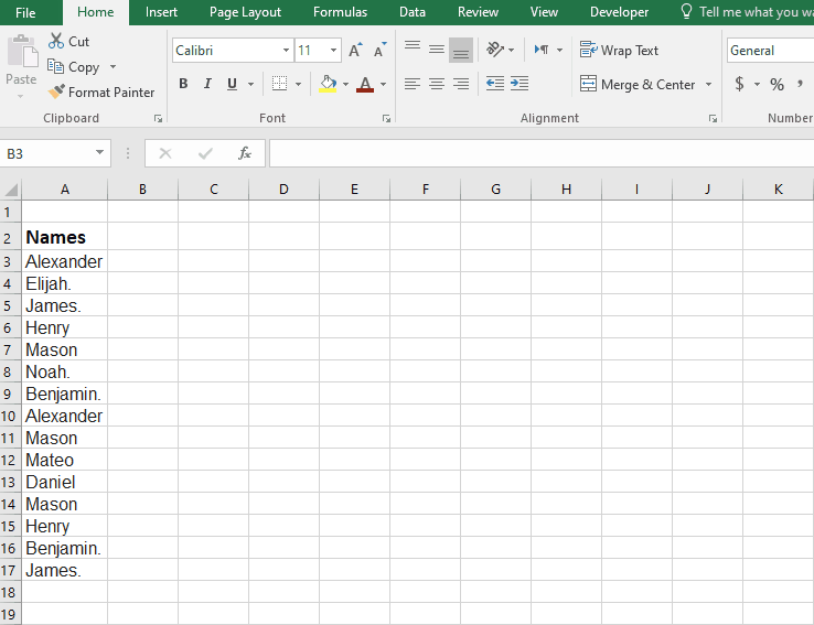
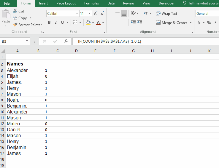
• Enter the formula “=IF(COUNTIF($A$3:$A$12,A3)=1,0,1)” next to the cell of available data.
• Press “F4” key to lock the column and row.

The COUNTIF formula checks in each cell of the available range whether the data repeats in another cell or not. The IF formula checks the result of COUNTIF. The $ sign is to lock the row and column. If the final result is 0, the data is unique and should be deleted and if the final result is 1, the data has its duplicate and should be kept.

• Drag down the cursor to apply the formula to the end of the available data as shown in the animation below:

Step 2 – Apply filter

• Now click on any cell where the formula is applied and go to the data option available at the above ribbon and click on filter.
• Click on the filter button available at the top, and now filter out the values which result in “0” because they are unique.

Step 3 – Delete the rows that are unique

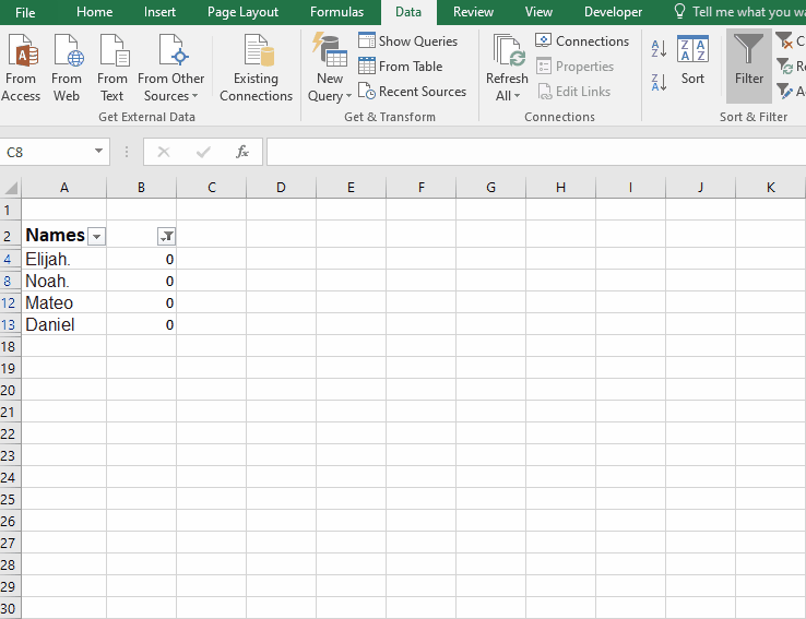
• Now select all visible filtered rows, right-click anywhere in the selected area and press select “delete” option.
• Now click on the filter button again and check Select All.
• Now the data will show only duplicate values as shown in the animation below:

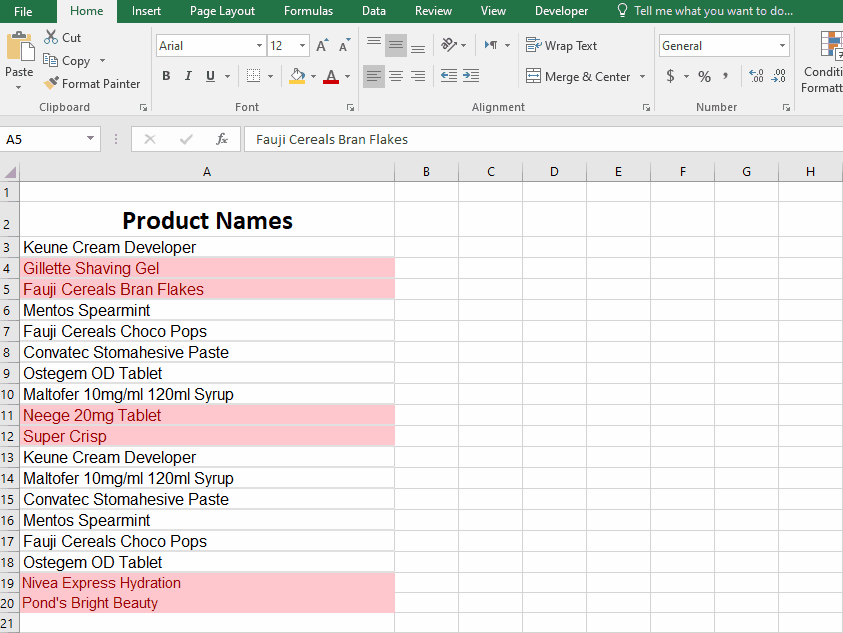
Method 2 – Using Conditional Formatting

Non Duplicate values can be removed by using the following steps, using proper conditional formatting. Follow the steps mentioned below to learn how to do it.

Step 1 – Select the range of cells and apply conditional formatting

• Select the range of cells that you want to check for duplicates.
• Click on the “Conditional Formatting” button in the “Home” tab of the ribbon.
• Choose “Highlight Cells Rules” and then “Duplicate Values” from the drop-down menu.
• In the “Duplicate Values” dialog box, select “Unique” from the drop-down menu under “Format all…”
• Click “OK” to close the dialog box and apply the formatting.

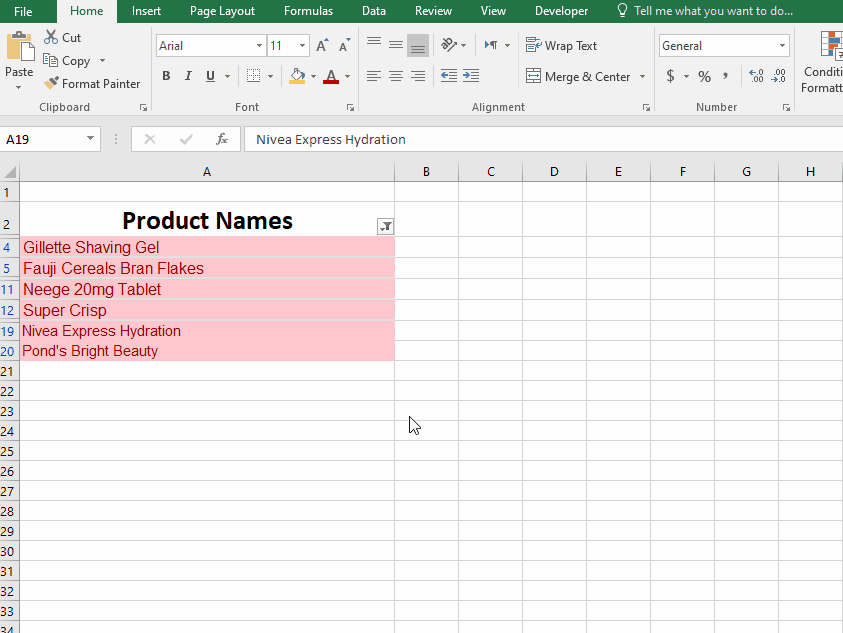
Step 2 – Apply filter by Cell Colour

• Now click on any cell where the formula is applied and go to the data option available at the above ribbon and click on filter.
• Click on the filter button available at the top, go to “Filter by color” and select “Filter by Cell Color”.
• The result will be unique items.

Step 3 – Delete the Filtered data

• Now select all visible filtered rows, right-click anywhere in the selected area, and press the “delete row” option.
• Now click on the filter button again and check Select All.
• Now the data will show only duplicate values as shown in the animation below: