How to remove duplicates but keep the first entry in Excel

Removing duplicates from data in Excel is important for a few reasons. Firstly, duplicate data can lead to inaccurate results and misrepresentation of the data. This is because when data is duplicated, the results of any calculations or analyses performed on the data will be skewed due to the duplicated values being counted multiple times. For example, if you are trying to find the average of a set of numbers and there are duplicates in the data, the average will not accurately reflect the true average of the set.

Secondly, having duplicate data can make it difficult to identify unique records or entries in the data. This can be a problem if you are trying to identify and analyze specific trends or patterns in the data, or if you are trying to combine or merge data from multiple sources. 

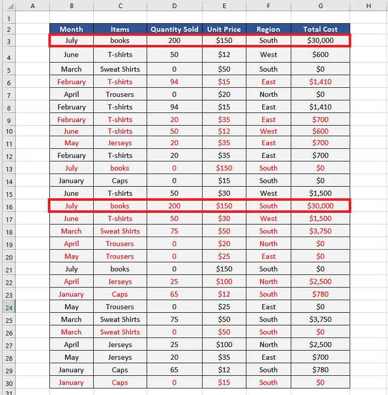
In this tutorial we are going to see how to achieve the goal of removing the duplicates while keeping the first entry intact. Let’s see the dataset below. We have intentionally entered duplicate values in the form of complete rows and highlighted one such example in the dataset shown above.

Let’s see how we can remove the duplicates while keeping the first one intact.

Option 1: Use built-in Remove Duplicates option

Step 1 – Select all data range

• Select all data rage first. To do this click on the first cell in the data range.
• Now while holding down CTRL+SHIFT press the right arrow and then down arrow to select the whole data range as shown above.

Step 2 – Use Remove Duplicates option from Data Menu

• Click on Data Tab from the main list of tabs.
• Now locate the Remove Duplicates option in the Data Tools group.
• Click on the Remove Duplicates command button.
• This will open the Remove Duplicates dialog box. It will ask you to select the column from which you want to remove the duplicates.
• Since we have intentionally entered the whole duplicate rows which means we have duplicates in each column of the data. Therefore, we’ll keep all columns checked and press the OK button.
• We’ll observe that the duplicates marked in red color are removed from the data and the original data i.e., the first entry is still intact as desired.

Option 2:  Use the Unique Function

Step 1 – Create the formula using UNIQUE function

• This one is probably the simplest of all solutions and we’ll need only one function i.e., UNIQUE. We’ll use the following formula to find only the unique values from the data.

=UNIQUE(B2:G30)

This will automatically keep only the first instance of all the duplicates and remove all other values as shown above. However, you will have to write this function somewhere outside your data range to get the results.

Option 3:  Use Power Query to remove duplicates

Step 1 – Import the data from Excel table / range

• Click on any cell in your data range.
• Now go to Data Tab from the main list of tabs.
• Locate the From Table/Range option in the Get & Transform Data group.
• Click on the action button From Table/Range. This will open up a create table dialog box. 
• By default, all data will be selected, however, if you want to change the range you can select a different data range by manual selection.
• If your data has headers then keep the checkbox in the dialog box checked as shown above and press OK. This will convert the data range into Excel table.

Step 2 – Remove duplicates using Power Query Editor

• This will open up the Power Query Editor and load all data in the editor.
• By default, only one column will be selected. Hold on the CTRL key and select all columns one by one.
• On the Home tab of Editor, go to the Reduce Rows group and click on Remove Rows action button.
• A dropdown menu will appear and choose Remove Duplicates. This will remove all the duplicates and only unique first instances will remain.
• Now click on the Close and Load action button. This will load the cleaned data in Excel as shown above.