How to protect columns in Google Sheets

In Google Sheets, protecting columns refers to the process of locking specific columns so that they cannot be edited or modified accidentally or intentionally by other users who have access to the same sheet. This can be particularly useful in situations where you are sharing a Google Sheet with others, and you want to ensure the integrity and security of certain columns.

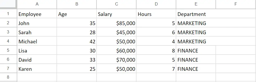
Our dataset comprises details related to a company’s employees, and their respective work hours and salaries. We aim to share this information with all the employees of the company while ensuring that no one can modify the data about the working hours and salaries. To achieve this, we will first select these specific columns and then utilize the ‘protect range’ feature to secure them.

Method 1: Protect Columns using the context menu options

Step 1 – Select the Columns

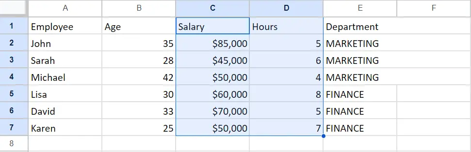
• Select the range of cells (columns) to be protected by using drag and drop method 

Step 2 – Open the Context menu

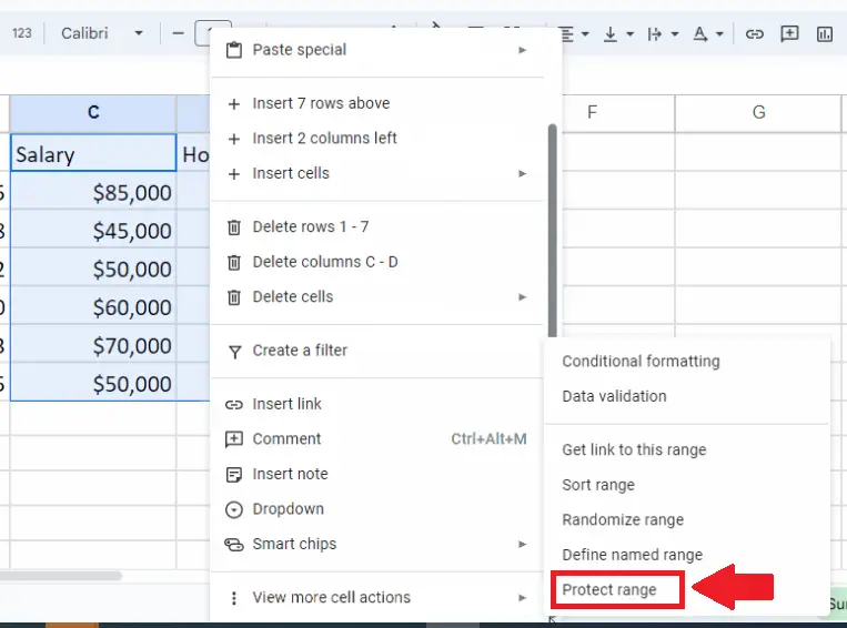
• After selecting the columns, right-click anywhere in the selected range and a context menu will appear

Step 3 – Click on the Protect range option

• In the context menu click on the “View More cell Actions” option and a right-side menu will appear
• From this right-side menu, Click on the Protect range option and a dialog box will appear on the right side of the sheet

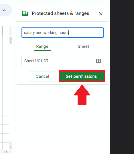
Step 4 – Type the Description

• In the dialog box type the name of columns in the “Enter Description” box 
• You may write any other description

Step 5 – Click on the Set Permissions option

• After typing the description, Click on the  Set Permissions option and a dialog box will appear

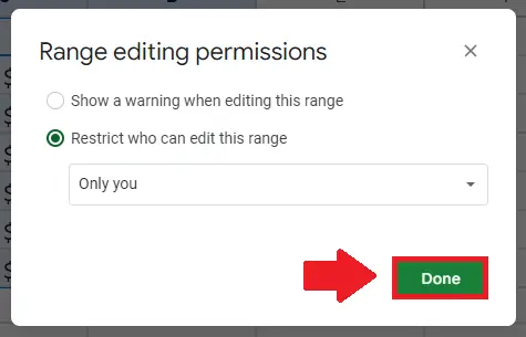
Step 6 – Set the Restriction

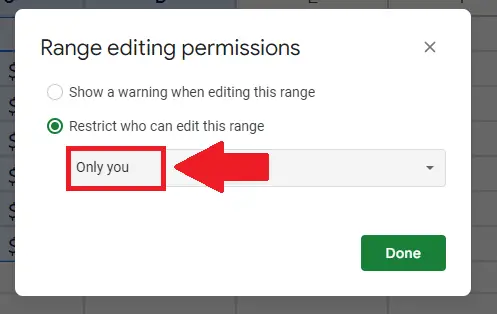
• In the dialog box, click on the check box of “Restrict who can edit this range” option 
• And select “ Only You” option in the box below it

Step 7 – Click on Done 

• After setting the restrictions, Click on Done at the end of the dialog box to save the changes made.

Method 2: Protect Columns using the Data tab

Step 1 – Select the Columns

• Select the range of cells (columns) to be protected by using drag and drop method 

Step 2 – Click on the Data tab

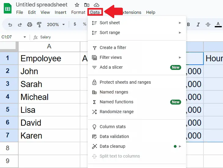
• After selecting the range of cells, click on the Data Tab from the taskbar and a drop-down menu will appear

Step 3 – Click on the Protect Sheets and Ranges option

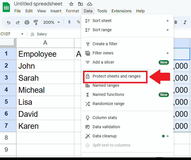
• From the drop-down menu, click on the  Protect Sheets and Ranges option and a dialog box will appear at the right side of the sheet

Step 4 – Type the Description

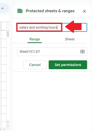
• In the dialog box type the name of columns in the “Enter Description” box 
• You may write any other description

Step 5 – Click on the Set Permissions option

• After typing the description, Click on the  Set Permissions option and a dialog box will appear

Step 6 – Set the Restriction

• In the dialog box, click on the check box of “Restrict who can edit this range” option 
• And select “ Only You” option in the box below it

Step 7 – Click on Done 

• After setting the restrictions, Click on Done at the end of the dialog box to save the changes made.