How to move cells down in Google Sheets

Moving cells down means shifting the content of one or more cells to the next row below. Moving cells down is an important function that allows you to manipulate the data in your spreadsheet to better organize and analyze it.

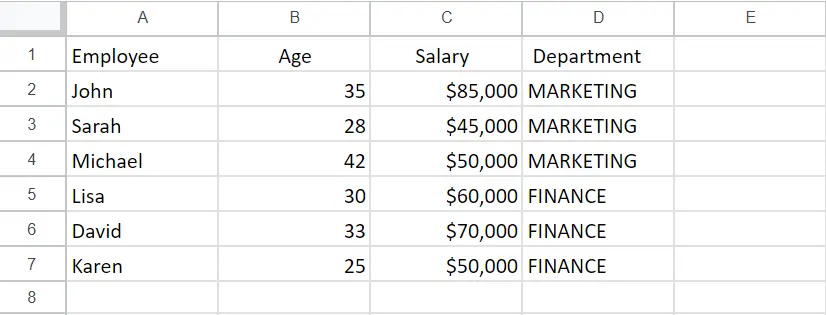
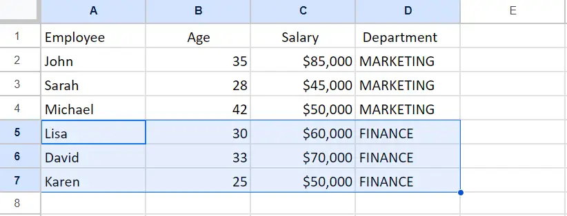
In our dataset, we have information on employees belonging to different departments of a company, specifically Marketing, and Finance. To segregate the employees according to their respective departments, we need to move the Finance department employees downwards. There are four different methods explained below to accomplish this task.

Method 1: Move Cells Down using the Insert Cells option

Step 1 – Select the Range of Cells

• Select the range of cells that you want to move down

Step 2 – Click on the Insert tab

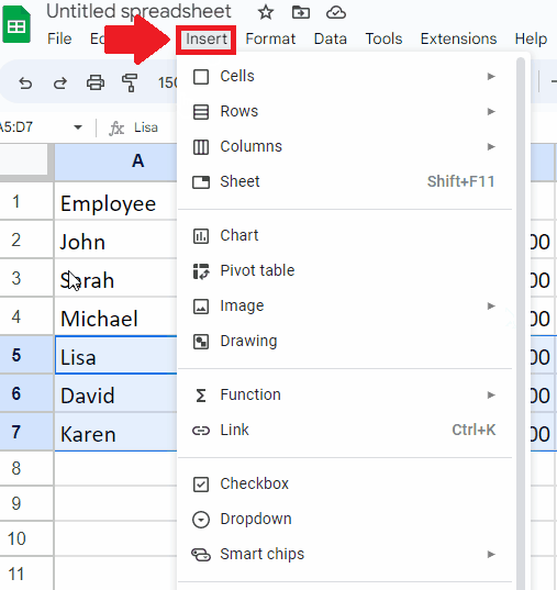
• After selecting the range of cells, click on the Insert tab, and a drop-down menu will appear

Step 3 – Click on the Insert 3 rows above option

• In the drop-down menu, click on Rows and a right-side menu will appear
• From this menu, click on the Insert 3 rows above option to get the required result

Method 2: Move cells down by Dragging

Step 1 – Select the Range of Cells

• Select the range of cells that you want to move down

Step 2 – Drag the Range 

• Move the cursor on the boundary of the selected range and drag it where you want to show the selected range 

Method 3: Move Cells down using the Context menu

Step 1 –  Select the Range of Cells

• Select the range of cells that you want to move down

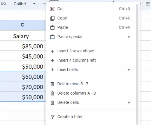
Step 2 – Open the context Menu

• After selecting the range of cells, right-click anywhere in the selected range and the context menu will appear

Step 3 – Click on the Insert 3 rows above option 

• In the context menu, Click on the Insert 3 rows above option to get the required result

Method 4: Move cells Down using Cut and Paste options

Step1 – Select the Range of Cells

• Select the range of cells that you want to move down

Step 2 – Open the Context menu

• After selecting the range of cells, right-click anywhere in the selected range and the context menu will appear

Step 3 – Click on the Cut option

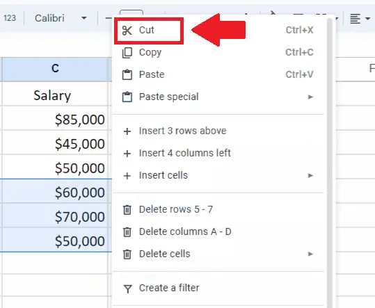
• In the Context menu, click on the Cut option

Step 4 – Select the Cell 

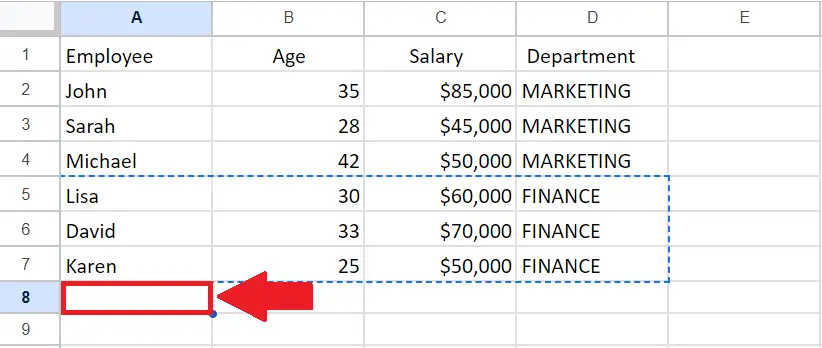
• Click on the cell where you want to show the selected range

Step 5 – Paste the selected Range

• Click on the selected cell and the context menu will appear
• From the context menu, click on the Paste option to get the required result