
How to match multiple columns in Excel
 By
SpreadCheaters
By
SpreadCheaters
There are numerous occasions in Excel where you need to compare four columns. When working with tiny tables, it is straightforward, but when comparing four columns in a huge spreadsheet, it becomes more challenging. Without the necessary information, you might have to manually compare the data or mark the rows of information that match or don’t match. With the use of some basic Excel understanding, this time-consuming method can be avoided.
This article examines each of the various ways that you might streamline this procedure. We’ll go over how to compare four columns with confidence and give instances of when doing so could be very helpful.
Method 1 – Using Conditional Formatting
Excel’s Conditional Formatting allows us to compare 4 columns. By using this approach, it is simple to find the duplicates.
Step – 1 – Select Data
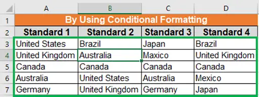
- Choose the 4 columns’ cells from the data collection.
Step – 2 – Go To Home Tab
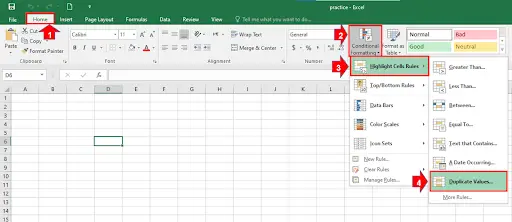
- Pick Conditional Formatting.
- From the Highlight Cells Rules menu, choose Duplicate Values.
Step – 3 – Apply Conditional Formatting
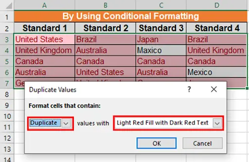
- By selecting the duplicate values, we will pop up below.
- From that pop up, we can create desired colours.
- Lastly, press “OK” button and get return.
Step – 4 – Duplicate Cells Highlighted
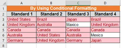
- Here, after comparing, we can observe that duplicate cells are coloured.
Method 2 – Use AND Function to match multiple columns
AND function is one of the very useful logical functions in Excel. It is employed to ascertain whether or not each test condition is TRUE. When all of its parameters are evaluated as TRUE, the AND function returns TRUE; otherwise, it returns FALSE.
Syntax
AND(logical_1, logical_2…)
logical 1: This one is the first condition or logical value to be assessed.
logical 2: This is the second predicate or logical value that needs to be assessed.
Result
If all of the conditions or logical values evaluate to true, it returns “true”.
If any of the conditions or logical values evaluate to false, it returns “false”.
Step – 1 – Add Helping Column
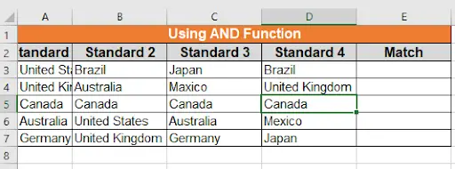
- Add the column “Match” in the dataset.
Step – 2 – Apply Formula
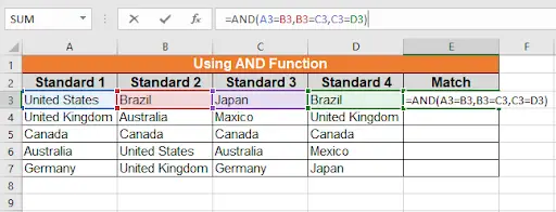
- Next, use AND function to compare each of the four cells in a column one at a time.
The formula is as below:
=AND(A3=B3,B3=C3,C3=D3)
- Press the Enter button.
Step – 3 – Drag The Formula
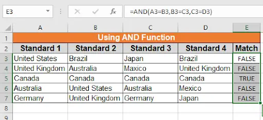
- Now drag down to apply formula on all rows, with help of selection handle.
- Below is the changes, we can find as per the requirements.
Method 3 – Match multiple Columns with COUNTIF Function
One of the statistical functions is the COUNTIF function. It is utilised to determine how many cells satisfy a requirement.
Syntax
COUNTIF(range,criteria)
Arguments:
range – specifies a cell or cells to count. The range is entered into a formula.
Criteria – the condition that tells the function which cells to count. It could be an expression, cell reference, text string, or number.
Step – 1 – Type The Formula
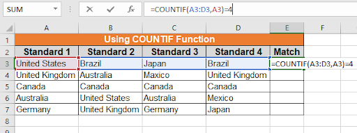
- Use the COUNTIF function to write the following formula in cell “E”:
=COUNTIF(A3:D3,A3)=4
- Press the enter button.
Step – 2 – Drag the Formula
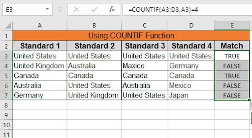
- Drag the formula downwards to apply on all rows, with the help of selection handle.
- The screen will look like below.
Method 4 – COUNTIF Function in another way
Step – 1 – Apply Formula
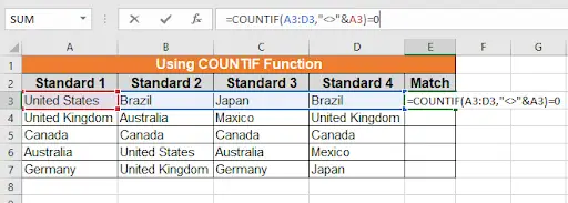
- Cell E3’s COUNTIF function should be modified. It goes like this:
- =COUNTIF(A3:D3,’’<>”&A3)=0
- Press the enter button.
Step – 2 – Drag the Formula
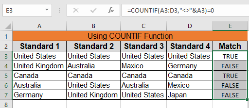
- Drag the formula below for application on all rows, with the help of selection handle.
- We can observe the required changes as show in below screen.


