How to sum duplicates in Excel

Excel is a powerful tool for managing data and performing calculations, but working with duplicates in large datasets can be tricky. Fortunately, Excel offers several built-in functions that can help you manage duplicate data, including the ability to Sum Duplicates.

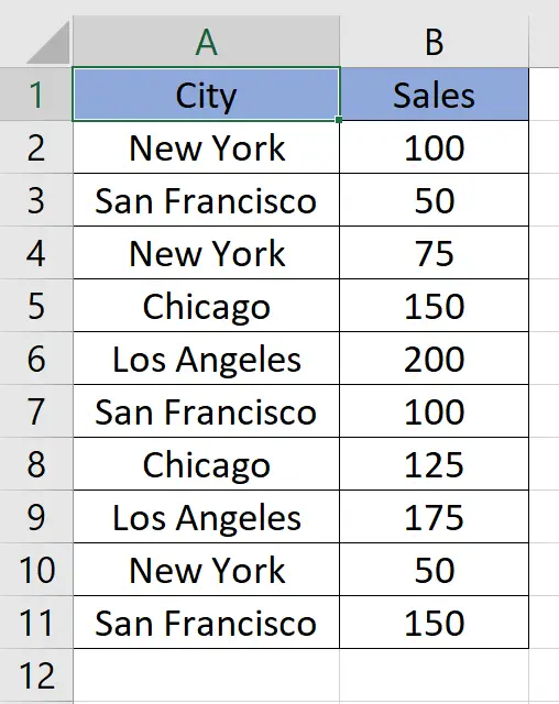
Here we have a dataset, in this dataset, there are the names of Cities and their Sales but there are also duplicates of some cities with different sales. In this tutorial, we will learn how to sum duplicates in excel but first let’s take a look at the Dataset above.

Method – 1 Using Pivot table.

Step – 1 Select the table.

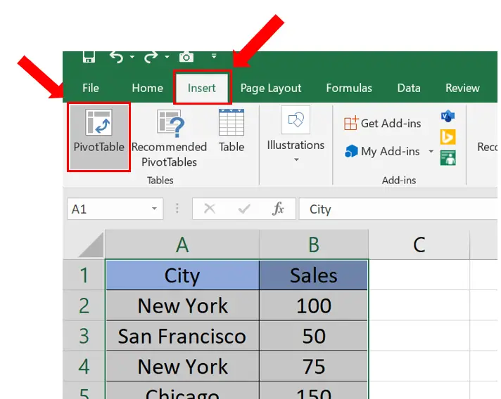
• Select the table which contains the duplicates.
• Go to the Insert tab.
• Click on the Pivot Table command in the Tables group.

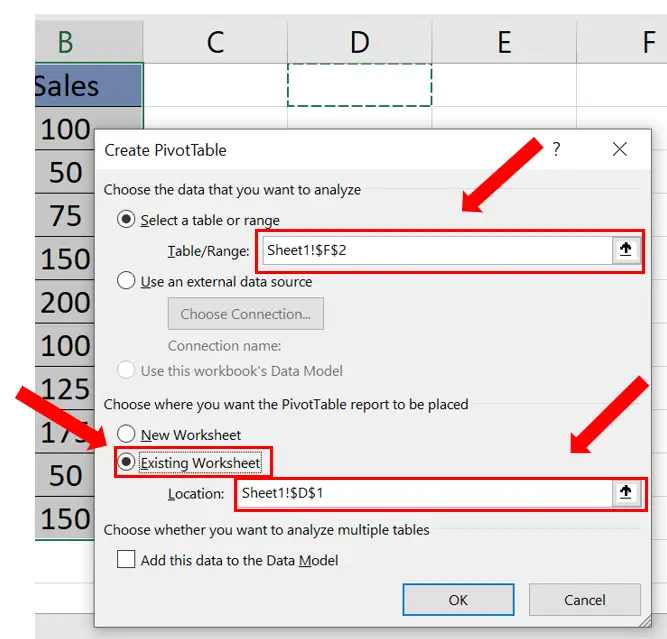
Step – 2 Insert the Pivot Table.

• Click on the Pivot Table command.
• The Create Pivot Table dialog box will.
• In the Table/Range menu select the table.
• Click on Existing Worksheet.
• Then select the cell where you want the Pivot Table in the Location menu.

Step – 3 Sum the duplicate.

• Clicking on Ok will create the Pivot Table.
• This will reveal the Pivot Table Fields dialog box.
• Click on the City and Sales tick box.
• Then choose City in the Rows dropdown list and Sum Of Sales in the Values dropdown menu.
• A table will be created containing the Sum of the duplicates and their Grand Total.

Method – 2 Using the SUMIF method.

Step – 1 Copying the column.

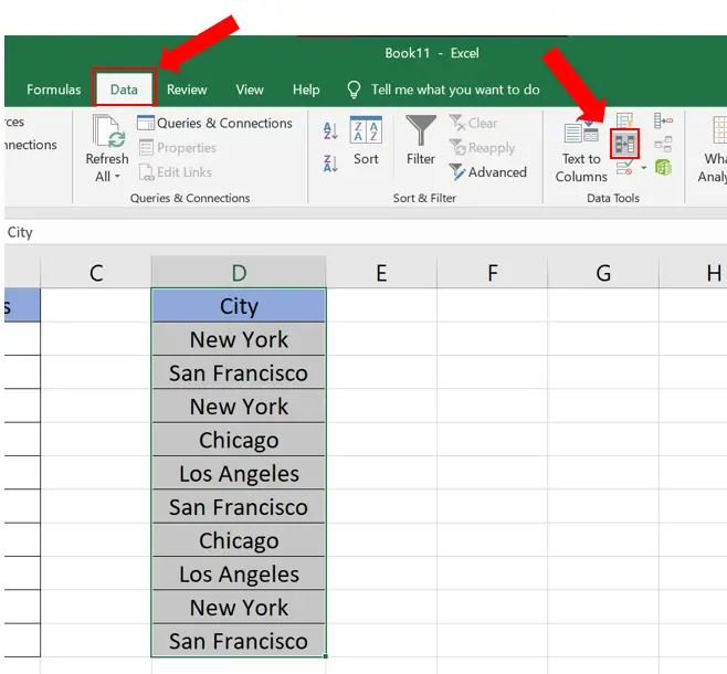
• Select the column containing the duplicates.
• Press Ctrl + C to copy the column then paste it into another column.
• Click on the Data tab.
• Click the Remove Duplicates command in the Data Tools group.

Step – 2 Removing Duplicates.

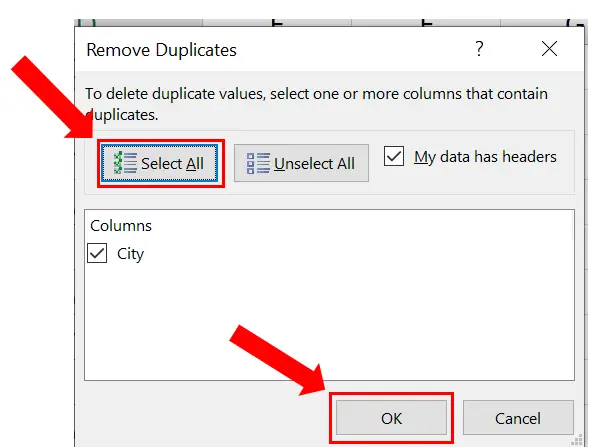
• Clicking on the Remove Duplicates command will reveal the Remove Duplicates dialog box.
• Click on Select All.
• Then click OK.

Step – 3 Use the SUMIF function.

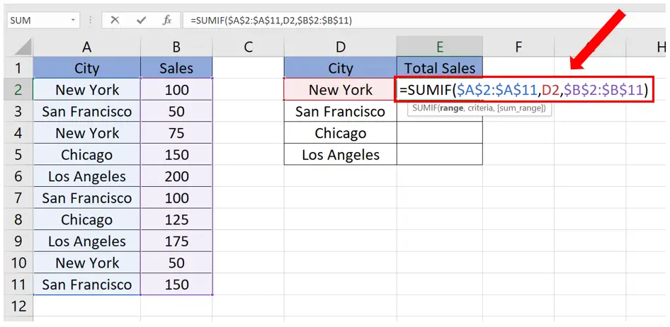
• Create another column for the total values.
• The syntax of the formula will be

=SUMIF(range, criteria, [sum_range])

• In our case the formula will be

=SUMIF($A$2:$A$11,D2,$B$2:$B$11)

Step – 4 Finding values of the rest of the cells.

• Select the cell with the formula.
• Drag from the bottom right down to the rest of the cells.
• The formula will be applied automatically.

Method – 3 Use the Consolidate tool.

Step – 1 Copy the Headers.

• Select the headers.
• Press Ctrl + C to copy the headers and then paste them into another column.
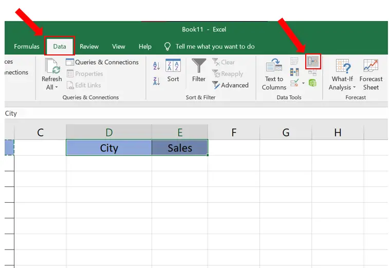
• Go to the Data tab.
• Click on the Consolidate command in the Data Tools group.

Step – 2 Adding the duplicates.

• Clicking on the Consolidate command will reveal the Consolidate dialog box.
• In the Reference box select the table you want to consolidate.
• Click on the Left column checkbox and then click OK.
• The duplicates will be added.