How To Make Vlookup Return Blank Instead Of 0

In this tutorial, we will show you step-by-step how to modify the VLOOKUP formula to return a blank cell when the lookup value is not found in the table. We will provide an example and walk you through the process, so you can easily implement this feature in your own Excel worksheets.

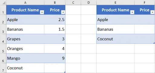
Suppose that we have a list of products with their prices and we want to create a VLOOKUP formula to find the price of a product based on its name. However, we want the formula to return a blank cell if the product price is not found in the list.

Here is a sample dataset:

Excel’s VLOOKUP function is a powerful tool for finding data in a table based on a specific lookup value. However, by default, when the lookup value is not found in the table, VLOOKUP returns a value of 0. This can be problematic, as it can result in incorrect calculations or confusion when working with large datasets. Fortunately, there is a simple solution to this issue: make VLOOKUP return a blank cell instead of 0 when a lookup value is not found.

Step 1 – Select Cell

– Select the cell where you want to type the formula. For our example, it’s F2.

Step 2 – Type Formula

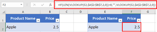
– Type the following formula.

=IF(LEN(VLOOKUP(E2,$A$2:$B$7,2,0))=0,””,VLOOKUP(E2,$A$2:$B$7,2,0)).

– Press enter to apply the formula to the cell.

Step 3 – Drag The Formula To The Remaining Cells

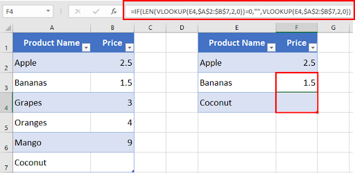
– Now drag the formula to the cells below.
– The formula returns the blank value for the product Coconut instead of ZERO.
– In the normal scenario, if the product name is found in the list, the price will be displayed as zero in column F. But in our case, the formula returned a blank cell.