
How to make the top row in Google Sheets stay
 By
SpreadCheaters
By
SpreadCheaters
Freezing the top row in Google Sheets means that the first row of the sheet remains in a fixed position on the screen, even when scrolling down. This keeps the column headings visible and is particularly useful when working with large datasets that have numerous rows. With the top row frozen, it’s easy to navigate the sheet while simultaneously referencing the column headings.
In this tutorial, we will learn how to make the top row in Google Sheets stay. Making the top row stay is a common task that can be achieved using the Freeze option in Google Sheets.
Currently, we have a dataset displaying sales of various products alongside the corresponding salespersons. Our objective is to make all the headers stay, which means that when we scroll vertically downward the headers are visible.
Method 1: Selecting the Top Row by Clicking the Column Header
Step 1 – Select the Top Row
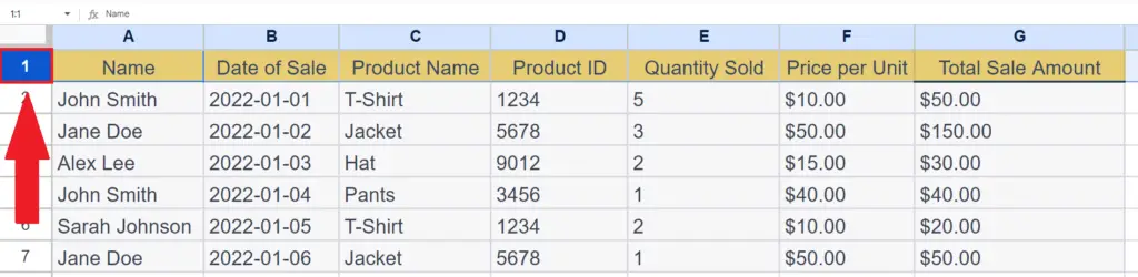
- Select the top row by clicking on the row header. This will select the complete row.
Step 2 – Locate the View Menu
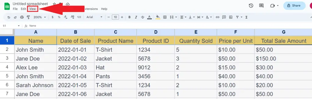
- Locate the View menu in the menu bar.
Step 3 – Choose the “Freeze” Option and Select “1 Row”
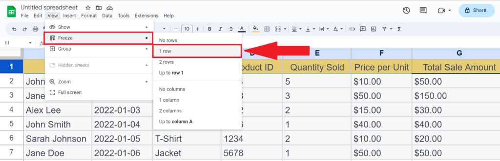
- Choose the “Freeze” option in the View drop-down menu and select “1 Row”.
- This will make the selected row stay.
Step 4 – Check Whether the Top Row Stays
- Scroll the sheet vertically to check if the top row stays.
Method 2: Utilizing the Blank Box on the Upper Left Corner of the Sheet
Step 1 – Hover the Cursor to the Horizontal Line of the Blank Box
- Hover the cursor on the horizontal boundary line of the block located at the upper-left corner of the sheet i.e. above the row headers and on the left of the column headers.
Step 2 – Click, Hold, and Drag the Cursor over the Rows You Want to Limit
- To limit the rows in Microsoft Excel, you can click and hold your mouse cursor on the column header of the first column i.e. the column with the row headers, and then drag it towards the right until it reaches the last row you want to limit.


