How to make the first column in Google Sheets Stay

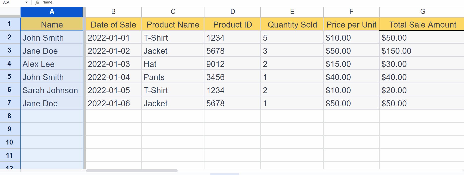
Making a column stay in Google Sheets allows you to lock it in place on the screen while scrolling horizontally. This is useful when working with a large dataset with multiple columns and you want to keep a specific column visible.

In this tutorial, we will learn how to make the first column in Google Sheets stay. Making a column stay is a common task that can be achieved using the Freeze option in Google Sheets. 

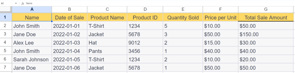
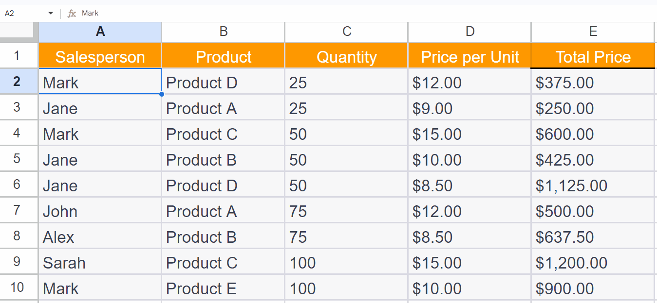
Currently, we have a dataset displaying sales of various products alongside the corresponding salespersons. Our objective is to keep the first column, which contains the names of the salespersons, fixed in position.

Method 1: Selecting the Column by Clicking the Column Header

Step 1 – Select the Column

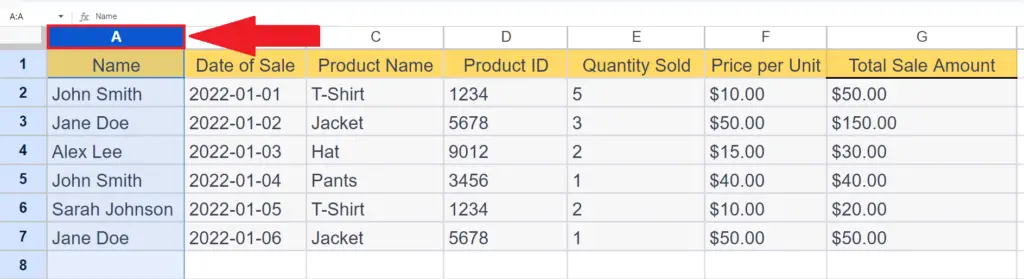
• Select the column by clicking on the column header.

Step 2 – Locate the View Menu

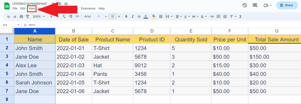
• Locate the View menu in the menu bar.

Step 3 – Choose the “Freeze” Option and Select “1 Column”

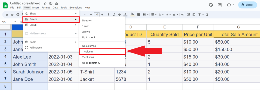
• Choose the “Freeze” option in the View drop-down menu and select “1 Column”.
• This will make the selected column stay.

Step 4 – Check Whether the First Column Stays

• Scroll the sheet horizontally to check if the column stays.

Method 2: Utilizing the Blank Box on the Upper Left Corner of the Sheet

Step 1 – Hover the Cursor to the Vertical Line of the Blank Box

• Hover the cursor on the vertical boundary line of the block located at the upper-left corner of the sheet i.e. above the row headers and on the left of the column headers.

Step 2 – Click, Hold, and Drag the Cursor over the Columns You want to Limit

• To limit the columns in Microsoft Excel, you can click and hold your mouse cursor on the column header of the first column i.e. the column with the row headers, and then drag it towards the right until it reaches the last column you want to limit.